General Description:
proximal subgradient method for solving problems of the form
Assumptions:
Available Oracles:
(the function values of f and g are not required in the economical setting)
Usage:
out               = prox_subgradient(Ffun,Ffun_sgrad,Gfun,Gfun_prox,lambda,startx,[par])
[out,fmin]        = prox_subgradient(Ffun,Ffun_sgrad,Gfun,Gfun_prox,lambda,startx,[par])
[out,fmin,parout] = prox_subgradient(Ffun,Ffun_sgrad,Gfun,Gfun_prox,lambda,startx,[par])
Input:
Ffun       - function handle for f
Ffun_sgrad - function handle for the subgradient of f
Gfun       - function handle for g (if g is extended real-valued, it is enough to specify the operation of g on its domain)
Gfun_prox  - function handle for the proximal mapping of g times a positive constant
lambda     - positive scalar
startx     - starting vector
par        - struct containing different values required for the operation of prox_subgradient
Output:out - optimal solution (up to a tolerance) fmin - optimal value (up to a tolerance) parout - a struct containing containing additional information related to the convergence. The fields of parout are: iterNum - number of performed iterations
funValVec - vector of all function values generated by the method Method Description:
Employs the proximal subgradient method for solving
using the following update scheme:
where
The method stops when at least one of the following conditions hold: (1) the number of iterations exceeded max_iter (2) the norm of the difference between two consecutive iterates is smaller than eps.
References:
Example 1:
Consider the problem
where A and b are given by
>> A = [0.6324 0.9575 0.9572 0.4218; 0.0975 0.9649 0.4854 0.9157; 0.2785 0.1576 0.8003 0.7922; 0.5469 0.9706 0.1419 0.9595];>> b = [0.6843; 0.6706; 0.4328; 0.8038];We solve the problem using prox_subgradient by taking f(x)=norm(A*x-b,1), lambda=2 and g(x)=norm(x,1). We use the fact that A'*sign(A*x-b) is a subgradient of f at x and the function prox_l1, which is part of the package (for a list of available prox functions, go here)
>> [out,fmin,parout] =prox_subgradient(@(x)norm(A*x-b,1),@(x)A'*sign(A*x-b),@(x)norm(x,1),@(x,a)prox_l1(x,a),2,zeros(4,1));*********************prox_subgradient*********************#iter fun. val. 6 2.526541 8 2.021784 10 1.869343 42 1.858085 152 1.845074 198 1.839026 214 1.826786 259 1.825962 347 1.825874 427 1.823920 500 1.821904 828 1.821805 901 1.820594 974 1.820261 ----------------------------------Optimal value = 1.820261 We can also plot the function values corresponding to the 1000 iterations of the method.
>> plot(parout.funValVec)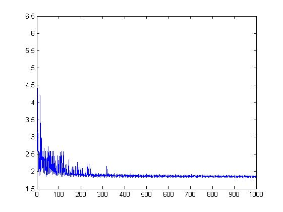 >> clear par>> par.max_iter=10000>> [out,fmin,parout] =prox_subgradient(@(x)norm(A*x-b,1),@(x)A'*sign(A*x-b),...@(x)norm(x,1),@(x,a)prox_l1(x,a),2,zeros(4,1),par);*********************prox_subgradient*********************#iter fun. val. 6 2.526541 8 2.021784 10 1.869343 42 1.858085 152 1.845074 : : 7290 1.816909 8311 1.816848 8632 1.816719 9974 1.816527 ----------------------------------Optimal value = 1.816527 We can obtain a slightly better solution by changing the parameter alpha controlling the stepsize of the method to 0.2 (the default is 1).
>> par.alpha=0.2;>> [out,fmin,parout] =prox_subgradient(@(x)norm(A*x-b,1),@(x)A'*sign(A*x-b),...@(x)norm(x,1),@(x,a)prox_l1(x,a),2,zeros(4,1),par);*********************prox_subgradient*********************#iter fun. val. 2 2.246688 3 1.965150 6 1.913995 8 1.868108 10 1.835076 31 1.834634 : : 4655 1.815429 5873 1.815387 7215 1.815360 7536 1.815359 8557 1.815340 8878 1.815321 ----------------------------------Optimal value = 1.815321 Example 2:
Consider the problem
where A is given by
>> randn('seed',315);>> A=randn(80,50);We construct the following MATLAB function (written as a separate m-file) which computes a subgradient of the objective function
function out=f_sgrad(x,A)[d,i]=max(A*x);out=A(i,:)';We now run the proximal subgradient method by calling for the prox_subgradient function with 10000 iterations.
>> clear par>> par.max_iter=10000;>> [out,fmin,parout] =prox_subgradient(@(x)max(A*x),@(x)f_sgrad(x,A),...@(x)0,@(x,a)proj_simplex(x),1,1/50*ones(50,1),par);*********************prox_subgradient*********************#iter fun. val. 344 0.340105 469 0.304347 773 0.295849 873 0.295266 1011 0.294499 1119 0.293705 1126 0.260861 1342 0.240381 1901 0.233554 2972 0.223986 3150 0.214869 3298 0.209238 4380 0.204554 4416 0.203054 4542 0.189647 5676 0.184367 5857 0.183907 6592 0.169232 7047 0.158440 ----------------------------------Optimal value = 0.158440 Note that the function g in this case is the indicator function. It is always enough to provide a function handle describing the operation of the function over its domain, and therefore in this case the input Gfun is the zeros function @(x)0. In addition, whenever g is an indicator function, the input lambda can be chosen to be any positive number. In the above, we picked it as 1, but any other positive number would give the same results.
The convergence of the method is actually rather slow. We can change the parameter par.alpha that controls the size of the stepsize of the method. For example, if we change the parameter from its default value (1) to 0.2, then a better solution is obtained.
>> par.alpha=0.2;>> [out,fmin,parout] =prox_subgradient(@(x)max(A*x),@(x)f_sgrad(x,A),@(x)0,@(x,a)proj_simplex(x),1,1/50*ones(50,1),par);*********************prox_subgradient*********************#iter fun. val. 17 0.322719 45 0.298787 91 0.285807 100 0.262558 113 0.254367 166 0.212918 202 0.210958 244 0.208830 273 0.184355 340 0.175955 403 0.159825 571 0.133207 909 0.124190 1467 0.112681 1763 0.108899 2331 0.108137 2376 0.108009 2389 0.107461 2397 0.093708 3793 0.086194 4069 0.085349 4570 0.085092 4997 0.082550 5675 0.081925 7103 0.074788 9926 0.074581 ----------------------------------Optimal value = 0.074581 Changing the alpha parameter to 1000 will cause the method to be slow at the extent that it will not produce a vector with better function value than the one of the initial vector. >> par.alpha=1000;>> [out,fmin,parout] =prox_subgradient(@(x)max(A*x),@(x)f_sgrad(x,A),@(x)0,...@(x,a)proj_simplex(x),1,1/50*ones(50,1),par);********************* prox_subgradient*********************#iter fun. val.----------------------------------Optimal value = 0.346508 In the setting of optimizing over the unit simplex, a different alternative for the proximal subgradient method is the CoMirror descent method. To run 10000 iterations of the method, we use the function comd.
>> clear parmd>> parmd.max_iter=10000;>> comd(@(x)max(A*x),@(x)f_sgrad(x,A),[],[],'simplex',1/50*ones(50,1),parmd);*********************Co-Mirror*********************#iter fun. val. 1 0.350156 2 0.312403 4 0.279940 5 0.259271 7 0.243640 9 0.204193 12 0.187565 15 0.186997 17 0.172044 21 0.156235 23 0.137774 34 0.121630 41 0.115435 45 0.114972 54 0.107758 62 0.096070 92 0.091377 96 0.086894 117 0.084414 136 0.080446 147 0.077282 199 0.074767 219 0.072659 234 0.069779 287 0.067462 311 0.067183 358 0.062960 381 0.061144 540 0.060613 624 0.059061 682 0.058997 787 0.057378 840 0.057114 945 0.056340 986 0.055261 1217 0.054538 1850 0.054488 1862 0.054259 1864 0.054216 1903 0.054068 2014 0.053233 2554 0.053072 2698 0.052960 2835 0.052414 2982 0.051827 4189 0.051738 4224 0.050887 6901 0.050879 7727 0.050688 9977 0.050557 ----------------------------------Optimal value = 0.050557 Obviously, a better solution was obtained.
|
Solvers >
