fdpg

Solvers‎ > ‎

General Description:

Fast dual proximal gradient method for solving problems of the form

$\min_x f(x)+\lambda g(Ax)$

Assumptions:

all functions are convex
f - strongly convex, closed and proper
g - proper closed and proximable
A - linear transformation
$\lambda$ - positive scalar

Available Oracles:

function value of f
gradient of the conjugate of f (meaning that for a given w, the oracle outputs argmax{<x,w>-f(x)})
function value of g
prox of a positive constant times g
value of the linear transformation A
value of the adjoint of A

(the function values of f,g are not required in the economical setting)

Usage:

out               = fdpg(Ffun,F_grad_conj,Gfun,Gfun_prox,Afun,Atfun,lambda,starty,[par])
[out,fmin]        = fdpg(Ffun,F_grad_conj,Gfun,Gfun_prox,Afun,Atfun,lambda,starty,[par])
[out,fmin,parout] = fdpg(Ffun,F_grad_conj,Gfun,Gfun_prox,Afun,Atfun,lambda,starty,[par])

Input:

Ffun - function handle for f (if f is extended real-valued, it is enough to specify the operation of f on its domain)

F_grad_conj - function handle for the gradient of the conjugate of f (for a given w, the oracle outputs argmax{<x,w>-f(x)})

Gfun - function handle for g (if g is extended real-valued, it is enough to specify the operation of g on its domain)

Gfun_prox - function handle for the proximal mapping of g times a positive constant

Afun - function handle for the linear transformation A
Atfun - function handle for the adjoint of the linear transformation A

lambda - positive constant
starty - starting vector of dual variables (resides in the image space of A)
par - struct containing different values required for the operation of fdpg

 field of par  possible values  default  description
  max_iter   positive integer  1000 maximal amount of iterations
eco_flag true/false   false true - economic version in which
function values are not computed 
 print_flag true/false   true true - internal printing is enabled
 Lstart positive real  1 an initial value for the Lipschitz constant
 const_flag  true/false  false true - constant stepsize is used
false - backtracking is employed
 regret_flag  true/false  false true - Lipschitz constant is divided by eta
       in the next iteration
false - otherwise
 real_valued_flag  true/false  false true  - g is assumed to be real-valued (only
        improved function values are printed)
false - otherwise
 feas_check_flag  true/false  true true - feasibility violation is printed
false - otherwise
 eta  real>1  2 multiplicative constant used when regretting
or backtracking
 eps  positive real  1e-5 stopping criteria tolerance (the
method terminates when

with x^k being the kth iterate vector)

Output:

out   - optimal solution (up to a tolerance)
fmin     - optimal value (up to a tolerance)
parout   - a struct containing containing additional information related to the convergence. The fields of parout are:

iterNum - number of performed iterations

funValVec - vector of all function values generated by the method
FeasValVec - vector of all feasibility violation values (relevant only when par.feas_check_flag=true)
LvalVec - vector of all used Lipschitz constants (relevant only when par.const_flag=true)
dualVec - dual optimal vector

Method Description:

Employs the fast dual proximal gradient method whose general update step is

$\begin{array}{ll} u^k &= {\rm argmax}_{u} \left \{ \langle u, A w^k \rangle -f(u) \right \};\\y^{k+1} &=w^k -\frac{1}{L_k} A u^k+\frac{1}{L_k} {\rm prox}_{\lambda L_k g}(A u^k-L_k w^k);\\t_{k+1} & =\frac{1+\sqrt{1+4t_k^2}}{2};\\w^{k+1} &=y^{k+1}+\left ( \frac{t_k-1}{t_{k+1}} \right ) (y^{k+1}-y^{k}).\end{array}$

where L_k is chosen either as a constant or by a backtracking procedure (default). The last computed vector u^k is considered as the obtained solution and the last computed y^k is the obtained dual vector.

References:

Amir Beck, "First Order Methods in Optimization", SIAM, 2017.
Amir Beck and Marc Teboulle, "A Fast Dual Proximal Gradient Algorithm for Convex Minimization and Applications", Operations Research Letters 42 (2014) 1-6.SIAM J. Optim. vol. 22 (2012), No. 2, 557--580.

Example 1:

Consider the problem of projecting a vector d on a polytope:

$\min \left \{ \frac{1}{2} \|x-d\|^2 : A x \leq b \right \}$

where d,A and b are generated as follows.

>> randn('seed',314);

>> A=randn(20,30);

>> b=randn(20,1);

>> d=randn(30,1);

To solve the problem, we will use the FDPG method with f, g and lambda are taken as

$f(x)=\frac{1}{2}\|x-d\|^2, g(x) = \delta_{\{y: y \leq b\}}(x), \lambda=1$

Note that since g is an indicator, lambda could have been chosen as any positive constant.

We can now run fdpg (the initial vector is of the same dimension as the image space of A)

>> [out,fmin,parout] = fdpg(@(x)0.5*norm(x-d)^2,@(x)x+d,@(x)0,@(x,a)min(x,b),@(x)A*x,@(x)A'*x,1,zeros(20,1));

*********************

fdpg

*********************

#iter fun. val. feas. viol. L val.

1 0.000000 12.8042 64.000000

2 0.657062 6.46853 64.000000

3 1.707604 2.85988 64.000000

4 2.479346 1.20314 64.000000

: : : :

74 2.754022 8.82372e-05 64.000000

75 2.754018 0.000152388 64.000000

76 2.754017 0.00019299 64.000000

77 2.754018 0.000207248 64.000000

Stopping because the norm of the difference between consecutive iterates is too small

----------------------------------

Optimal value = 2.754018

Note that the Gfun_prox input was computed by the formula min(x,b) since

${\rm prox}_{a g}(x)={\rm prox}_{a \delta_{\{y: y \leq b\}}}(x)=P_{\{y: y \leq b\}}(x) = \min\{x,b\}$

The formula for the F_grad_conj is a result of the following computation:

${\rm argmax}_{y} \left \{ \langle x,y \rangle -f(y) \right \}={\rm argmax}_{y} \left \{ \langle x,y \rangle -\frac{1}{2}\|y-d\|^2 \right \}=x+d$

The constraint violation of the obtained solution can be computed by

>> norm(max(A*out-b,0))

ans =

2.072481037126269e-04

which is obviously the same as

>> parout.feasVal(end)

ans =

2.072481037126269e-04

The maximal amount of iterations by default is 1000, but the algorithm stopped after 77 iterations since the difference between consecutive iterates was too small. To enforce the method to run for more than 77 iterations, we can change the parameter eps that controls the upper bound on the distance between consecutive iterates (whose default is 1e-5)

>> clear par

>> par.eps=1e-8;

>> [out,fmin,parout]=fdpg(@(x)0.5*norm(x-d)^2,@(x)x+d,@(x)0,@(x,a)min(x,b),@(x)A*x,@(x)A'*x,1,zeros(20,1),par);

*********************

fdpg

*********************

#iter fun. val. feas. viol. L val.

1 0.000000 12.8042 64.000000

2 0.657062 6.46853 64.000000

3 1.707604 2.85988e 64.000000

4 2.479346 1.20314 64.000000

5 2.822158 0.590423 64.000000

6 2.903982 0.283675 64.000000

7 2.879172 0.141183 64.000000

8 2.835106 0.0841442 64.000000

: : : :

148 2.754038 7.87737e-07 64.000000

149 2.754038 1.12641e-06 64.000000

150 2.754038 1.29568e-06 64.000000

151 2.754038 1.29757e-06 64.000000

Stopping because the norm of the difference between consecutive iterates is too small

----------------------------------

Optimal value = 2.754038

Obviously, more iterations were performed under the new tolerance parameter. Note also that although the obtained function value is slightly higher than the one obtained with eps=1e-5, the feasibility violation of the obtained solution is significantly better.

Example 2:

Consider the following denoising problem:

$\min \left \{\frac{1}{2} \sum_{i=1}^{1000} (x_i-y_i)^2+4 \sum_{i=1}^{999} |x_i-x_{i+1}| \right \}$

where y is a noisy step function generated as follows.

>> randn('seed',314);

>> x=zeros(1000,1);

>> x(1:250)=1;

>> x(251:500)=3;

>> x(751:1000)=2;

>> y=x+0.05*randn(size(x));

The "true" and noisy signals can be plotted.

>> figure(1)

>> subplot(1,2,1)

>> plot(1:1000,x,'.')

>> subplot(1,2,2)

>> plot(1:1000,y,'.')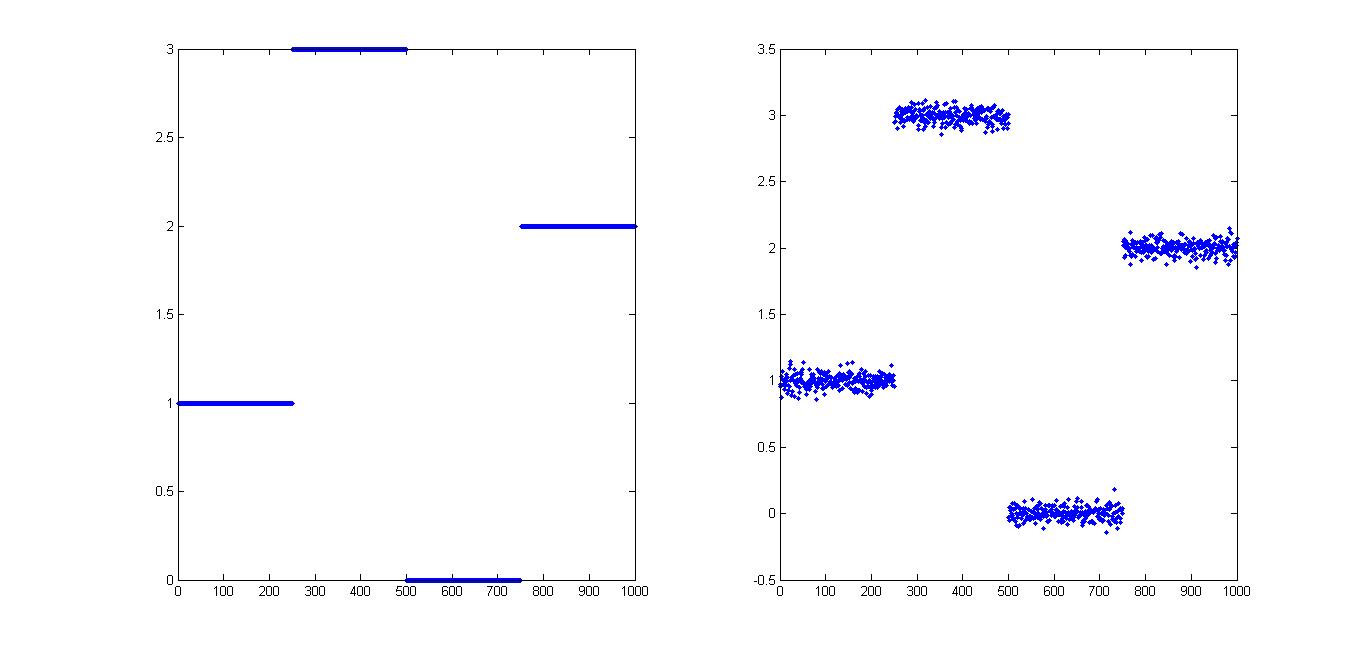

The problem can be rewritten as

$\min_x f(x)+4 g(Ax)$

where

$f(x)=\frac{1}{2}\|x-y\|_2^2, g(z)=\|z\|_1 \; (z \in {\mathbb R}^{999})$

and A given by

>> A=sparse(999,1000);

>> for i=1:999

>> A(i,i)=1;

>> A(i,i+1)=-1;

>> end

We can now solve the problem using fdpg

>> [out,fmin,parout] = fdpg(@(x)0.5*norm(x-y)^2,@(x)x+y,@(x)norm(x,1),@(x,a)prox_l1(x,a),@(x)A*x,@(x)A'*x,4,zeros(999,1));

*********************

fdpg

*********************

#iter fun. val. feas. viol. L val.

1 248.511179 3.1607e-07 4.000000

2 107.310785 3.1607e-07 4.000000

3 74.301824 3.1607e-07 4.000000

4 60.396805 3.1607e-07 4.000000

5 53.851067 3.1607e-07 4.000000

996 28.915146 3.15595e-07 4.000000

997 28.909778 3.15432e-07 4.000000

998 28.904498 3.14599e-07 4.000000

999 28.899496 3.13701e-07 4.000000

1000 28.895505 3.13267e-07 4.000000

----------------------------------

Optimal value = 28.895505

Since the function g is real-valued, it is better to invoke the function with real_valued_flag set to true, since in this case there is no need to check for feasibility violation and the algorithm outputs the iterate with the smallest function value.

>> clear par

>> par.real_valued_flag=true;

>> [out,fmin,parout] = fdpg(@(x)0.5*norm(x-y)^2,@(x)x+y,@(x)norm(x,1),@(x,a)prox_l1(x,a),@(x)A*x,@(x)A'*x,4,zeros(999,1),par);

*********************

fdpg

*********************

#iter fun. val. L val.

2 107.310785 4.000000

3 74.301824 4.000000

4 60.396805 4.000000

5 53.851067 4.000000

6 50.175863 4.000000

7 48.060216 4.000000

8 46.621121 4.000000

9 45.632373 4.000000

10 45.103918 4.000000

11 44.149710 4.000000

15 43.972166 4.000000

: : :

496 28.942826 4.000000

497 28.926443 4.000000

498 28.910757 4.000000

499 28.899488 4.000000

500 28.892469 4.000000

----------------------------------

Optimal value = 28.892469

The last recorded iteration is 500 since there was no improvement of function value following that iteration (although 1000 iterations were employed).

Note also that a slightly smaller function value was obtained in this case. The obtained solution is an excellent reconstruction of the original signal.

>> figure(2);

>> plot(1:1000,out,'.')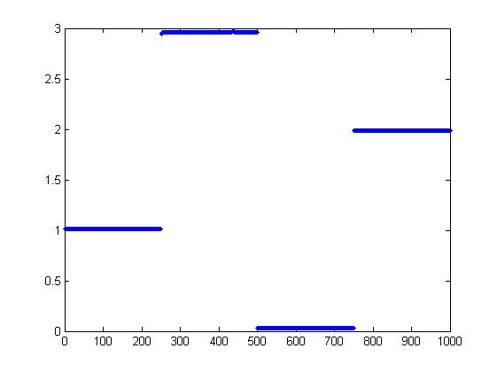

Example 3:

Consider the problem

$\min_{X \in {\mathbb R}^{30 \times 40}} \left \{ \frac{1}{2} \|C \odot (X-D)\|_F^2+\|A X B\|_F\right \}$

where

$C,D \in {\mathbb R}^{30 \times 30}, A \in {\mathbb R}^{20 \times 30}, B \in {\mathbb R}^{40 \times 50}$

and $\odot$ stands for the Hadamard product (coordinate-wise multiplication) of two matrices of the same size.

The matrices A,B,C,D are generated as follows.

>> randn('seed',314);

>> rand('seed',314);

>> A=randn(20,30);

>> B=randn(40,50);

>> C=1+rand(30,40);

>> D=randn(30,40);

To solve the problem, we will use the FDPG method with lambda=1,

$f(X)= \frac{1}{2} \|C \odot (X-D)\|_F^2, g(Y) = \|Y\|_F$

and the linear transformation being $X \mapsto A X B$ . Note that since C has only nonzero components, it follows that f is strongly convex as required. In employing the FDPG method, we will use the following facts:

the adjoint linear transformation is given by $Y \mapsto A^T Y B^T$
the gradient of the conjugate of f is given by

$\nabla f^*(Y) = {\rm argmax}_{X} \{ \langle X,Y \rangle - f(X) \}=E \odot Y+D$

where E is the matrix defined by

$E_{ij}=\frac{1}{C_{ij}^2}, i=1,2,\ldots,30, j=1,2,\ldots,40$

The command invoking fdpg is

>> E = 1./(C.^2);

>> clear par

>> par.real_valued_flag=true;

>> [out,fmin,parout] = fdpg(@(X)0.5*norm(C.*(X-D),'fro')^2,@(X)E.*X+D,...

@(X)norm(X,'fro'),@(x,a)prox_Euclidean_norm(x,a),@(X)A*X*B,@(X)A'*X*B',1,zeros(20,50),par);

*********************

fdpg

*********************

#iter fun. val. L val.

2 693.740808 4096.000000

3 623.515605 4096.000000

6 553.714050 8192.000000

: : :

279 485.921545 8192.000000

280 485.921545 8192.000000

281 485.921545 8192.000000

282 485.921545 8192.000000

283 485.921545 8192.000000

Stopping because the norm of the difference between consecutive iterates is too small

----------------------------------

Optimal value = 485.921545