comd

Solvers‎ > ‎

General Description:

CoMirror descent for solving problems of the form

$\min \{f(x):g(x)\leq 0, x\in X\}$

Assumptions:

f and the components of g (g₁,g₂,...,g_m) are convex and Lipschitz
X is one of the following four sets:

simplex $\left \{x: \sum_{i=1}^n x_i =r (\leq r), \ell_i \leq x_i \leq u_i\right \}$

l₂-norm ball $\{x: \|x-c\|\leq r \}$

box $\{x: \ell_i \leq x_i \leq u_i, i=1,2,\ldots,n \}$

spectahedron $\{X \in \mathbb{S}^n : 0 \preceq X \preceq u I, {\rm Tr}(X)=r (\leq r) \}$

The settings of l₂-norm ball and box also handle the situation of matricial decision variables. In this case, the function operates on mxn matrices in the same way it operates on the corresponding m*n-length column vector.

Available oracles:

function value of f
subgradient of f
function values of the components of g
subgradients of the components g

(the function value of f is not required in the economical setting)

Usage:

out               = comd(Ffun,Ffun_sgrad,Gfun,Gfun_sgrad,set,startx,[par])
[out,fmin]        = comd(Ffun,Ffun_sgrad,Gfun,Gfun_sgrad,set,startx,[par])
[out,fmin,parout] = comd(Ffun,Ffun_sgrad,Gfun,Gfun_sgrad,set,startx,[par])

Important remark: comd can be run without constraints. In such cases, Gfun and Gfun_sgrad should be replaced by []

Input:

Ffun       - function handle for the objective function f
Ffun_sgrad - function handle for the subgradient of the objective function f
Gfun       - function handle for the constraint function g
Gfun_sgrad - function handle for the subgradients of the components of the constraint function (arranged in columns)
set        - underlying set; allowed values: 'simplex', 'ball','box','spectahedron'
startx     - starting vector
par        - struct containing different values required for the operation of comd:

 field of par  possible values  default  description
  max_iter   positive integer  1000 maximal amount of iterations
eco_flag true/false   false true - economic version in which
function values are not computed 
 print_flag true/false   true true - internal printing is enabled
 stuck_iter positive integer  10000 maximal allowed number of iterations
without improvement of function
value
 feas_eps  positive real  1e-5 allowed feasibility violation
simplexR 
(set='simplex') real   1  "radius" of the simplex set
 specR
(set='spectahedron')
 positive real  1 radius of the spectahedron 
 ballR
(set='ball')  positive real  1 radius of the ball
 ballCenter
(set='ball')  real vector  zeros
vector center of the ball
 isequal
(set='simplex'/'spectahedron)  true/false  true true if equality is imposed, otherwise
false 
 lowb 
(set='simplex' or 'box')
real vector/scalar   0 lower bounds on the variables
upb 
(set='simplex') extended real
vector
(Inf is allowed)   Inf upper bounds on the variables

upb
 (set='spectahedron')  positive real
or Inf  Inf upper bound on the eigenvalues

 upb 
(set='box')  real vector/scalar  1 upper bound on the variables

Output:

out - optimal solution (up to a tolerance)
fmin - optimal value (up to a tolerance)
parout - a struct containing containing additional information related to the convergence. The fields of parout are:

iterNum - number of performed iterations

funValVec - vector of all function values generated by the method

consVec - vector containing all the constraints violations quantities

Method Description:

Employs the CoMirror method for solving

$\min \{f(x):g(x)\leq 0, x\in X\}$

using the following update scheme:

$x^{k+1} = {\rm argmin} \{ \langle t_k e_k -\nabla \omega(x^k),x\rangle +\omega(x):x \in X\}$

$e_k = \left \{ \begin{array}{ll} f'(x^k), & \tilde{g}(x^k) \leq \varepsilon,\\\tilde{g}'(x^k),& \mbox{else}, \end{array} \right.$

where t_k is a stepsize and

$\tilde{g}(x)=\max\{g_1(x),g_2(x),\ldots,g_m(x)\}$

The function $\omega$ is determined by the identity of X.

X	$\omega$
box/ball	$\omega(x)=\frac{1}{2}\\|x\\|_2^2$
simplex	$\omega(x)=\sum_i x_i \log(x_i)$
spectahedron	$\omega(X)=\sum_i \lambda_i(X) \log(\lambda_i(X))$

The method stops when at least one of the following conditions hold: (1) the number of iterations exceeded max_iter (2) the function value at feasible points did not improve in stuck_iter iterations.

References:

Amir Beck, Aharon Ben-Tal, Nili Guttmann-Beck and Luba Tetruashvili, The CoMirror algorithm for solving nonsmooth constrained convex problems, Operations Research Letters, volume 38, issue 6 (2010), 493-–398.
Amir Beck, "First Order Methods in Optimization", SIAM, 2017.
Amir Beck and Marc Teboulle, Mirror descent and nonlinear projected subgradient methods for convex optimization , Oper. Res. Lett. 31 (2003), no. 3, 167--175.
Aharon Ben-Tal, Tamar Margalit and Arkadi Nemirovsi, The ordered subsets mirror descent optimization method with applications to tomography, SIAM J. Optim. (2001), volume 12, no. 1, 79--108.

Example 1:

Consider the problem

$\min \{ \|Ax-b\|_1 : x \in \Delta_{100}\}$

where A and b are generated by the commands

>> randn('seed',315);

>> A=randn(40,100);

>> b=randn(40,1);

An optimal solution of the problem can be found by the CoMirror method by the following commands

>> f = @(x)norm(A*x-b,1);

>> f_grad = @(x)A'*sign(A*x-b);

>> [out,fmin]=comd(f,f_grad,[],[],'simplex',zeros(100,1));


*********************
Co-Mirror
*********************
 #iter        fun. val.
     1         34.369794 
     2         31.413493 
     3         29.956959 
     4         29.062173 
     :              :

   626         27.286224 
   644         27.286194 
   661         27.282972 
   673         27.281621 


----------------------------------
optimal value =       27.281621

Note that we set the initial vector to be the zeros vector. In addition, the solver only prints information on iterations in which the function value improved.

The optimal solution and optimal value are stored in the output variables out and fmin

>> out

out =

0.0000

0.0806

0.0000

0.0098

:

0.0000

>> fmin

fmin =

27.2816

To plot the function values of the sequence generated by the method the following commands should be executed.

>> [out,fmin,parout]=comd(f,f_grad,[],[],'simplex',zeros(100,1));

>> plot(1:length(parout.funValVec), parout.funValVec)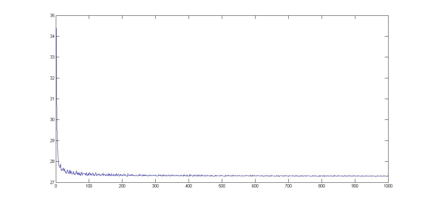

A better solution can be reached if more iterations are employed.

>> par.max_iter=10000;

>> [out,fmin]=comd(f,f_grad,[],[],'simplex',zeros(100,1),par);

*********************

Co-Mirror

*********************

#iter fun. val.

1 34.369794

2 31.413493

3 29.956959

4 29.062173

: :

8660 27.272538

9467 27.272437

9650 27.272244

9993 27.271796

----------------------------------

Optimal value = 27.271796

Example 2:

Consider the problem

$\begin{array}{ll} \min & c_1x_1+c_2 x_2\\ \mbox{s.t.} & x_1 A_1+x_2 A_2 \preceq I,\\ & x_1^2 +x_2^2 \leq 1. \end{array}$

Here A1 and A2 are 10x10 symmetric matrices. To solve the problem using comd, we first reformulate it as

$\begin{array}{ll} \min & f(x_1,x_2)\equiv c_1x_1+c_2x_2,\\ \mbox{s.t.} & g(x_1,x_2)\equiv \lambda_{\max}(x_1A_1+x_2A_2-I)\leq 0,\\ & x \in X=B[0,1]. \end{array}$

c1,c2,A1,A2 are generated by the commands

>> randn('seed',316);

>> A1=randn(10,10);

>> A1=(A1+A1')/2;

>> A2=randn(10,10);

>> A2=(A2+A2')/2;

>> c=[1;1];

A subgradient of g can be computed by the formula [v'*A1*v;v2'*A2*v], where v is a normalized eigenvector corresponding to the maximum eigenvalue of x(1)*A1+x(2)*A2-eye(10). This computation is performed in the following MATLAB function (written as a separate m-file)

function out=sgrad_eig(x,A1,A2);

[v,d]=eigs(x(1)*A1+x(2)*A2-eye(size(A1)),1,'la');

out=[v'*A1*v;v'*A2*v];

We can now solve the problem using comd

>> f = @(x)c'*x

>> f_sgrad = @(x)c

>> g=@(x)eigs(x(1)*A1+x(2)*A2-eye(10),1,'la');

>> g_sgrad=@(x)sgrad_eig(x,A1,A2);

>> [out,fmin]=comd(f,f_sgrad,g,g_sgrad,'ball',zeros(2,1));


*********************
Co-Mirror
*********************
#iter        fun. val.      con. val.
     2         -0.027117     -0.388949
     4         -0.182910     -0.329495
     6         -0.261001     -0.200118
     8         -0.309909     -0.109328
     :             :                    :
   628         -0.387209     -0.000002
   634         -0.387210     -0.000000
   640         -0.387211      0.000002
   646         -0.387212      0.000003
   652         -0.387212      0.000005
   658         -0.387213      0.000007
   664         -0.387214      0.000009
----------------------------------
Optimal value =       -0.387214

The optimal solution is

>> out

out =

-0.1539

-0.2333

Note that that the obtained solution slightly violates the constraint (the maximum eigenvalue is 0.000009). If it is imperative that to avoid any violation of constraints we set the parameter par.feas_eps to 0.

>> clear par

>> par.feas_eps=0;

>> [out,fmin]=comd(f,f_sgrad,g,g_sgrad,'ball',zeros(2,1),par);

*********************

Co-Mirror

*********************

#iter fun. val. con. val.

2 -0.027117 -0.388949

4 -0.182910 -0.329495

6 -0.261001 -0.200118

8 -0.309909 -0.109328

: : :

664 -0.387207 -0.000009

670 -0.387208 -0.000007

676 -0.387209 -0.000005

682 -0.387209 -0.000003

688 -0.387210 -0.000001

----------------------------------

Optimal value = -0.387210

Example 3:

Consider the problem

$\begin{array}{ll} \min & \lambda_{\max}(X+C) +{\rm Tr}(DX) \\ \mbox{s.t.} & {\rm Tr}(C_1 X) \leq 0.6, \\ & {\rm Tr}(C_2 X) \leq 0, \\ & {\rm Tr}(X)=0.2, \\ & X \succeq 0. \end{array}$

where C,D,C₁,C₂ are given by

>> C = [2.5629 1.2010 0.4374 1.0687

1.2010 0.0511 0.4333 -0.5491

0.4374 0.4333 1.0602 -2.1081

1.0687 -0.5491 -2.1081 0.0795];

>> D = [0.6516 0.7271 1.0526 1.2098

0.7271 0.5108 0.9531 1.5011

1.0526 0.9531 0.3270 1.3611

1.2098 1.5011 1.3611 0.5152];

>> C1 =[0.8328 -0.1293 -0.4879 0.8372

-0.1293 0.8967 0.6505 -0.0566

-0.4879 0.6505 -0.6712 0.5950

0.8372 -0.0566 0.5950 0.3656];

>> C2 =[3.5267 0.2487 -0.6312 0.7461

0.2487 -0.6479 0.9198 -0.2510

-0.6312 0.9198 -1.0649 -0.5603

0.7461 -0.2510 -0.5603 -0.3176];

To solve the problem, we first construct the following MATLAB function (written as a separate m-file) which computes a subgradient of the objective function

function out=f_sgrad(X,C,D)

a=X+C;

a=(a+a')/2;

[v,d]=eigs(a,1,'la');

out=v*v'+D;

We can now solve the problem using comd

>> f=@(X)eigs((X+X')/2+C,1,'la')+trace(D*X);

>> clear par

>> par.specR=0.2;

>> [out,fmin]=comd ( f ,@(X) f_sgrad(X,C,D) ,@(X)[trace(C1*X)-0.6;trace(C2*X)], @(X)[C1,C2],'spectahedron',ones(4,4),par) ;

*********************

Co-Mirror

*********************

#iter fun. val. con. val.

25 4.099380 -0.000781

26 4.098417 -0.002056

27 4.097445 -0.003327

28 4.096465 -0.004593

29 4.095478 -0.005854

30 4.094484 -0.007110

: : :

973 3.037749 0.000007

978 3.037720 -0.000028

983 3.037691 -0.000063

988 3.037663 -0.000097

993 3.037636 -0.000132

998 3.037609 -0.000166

----------------------------------

Optimal value = 3.037609

The default for the feasibility violation is 1e-5. We can relax it to a smaller value, say 1e-3,

>> par.feas_eps=1e-3

>> [out,fmin]=comd ( f ,@(X) f_sgrad(X,C,D) ,@(X)[trace(C1*X)-0.6;trace(C2*X)], @(X)[C1,C2],'spectahedron',ones(4,4),par) ;

*********************

Co-Mirror

*********************

#iter fun. val. con. val.

25 4.099380 -0.000781

26 4.098417 -0.002056

27 4.097445 -0.003327

28 4.096465 -0.004593

29 4.095478 -0.005854

: : :

977 3.037426 0.000994

982 3.037398 0.000957

987 3.037370 0.000921

992 3.037343 0.000884

997 3.037317 0.000849

----------------------------------

Optimal value = 3.037317

Note that the output solution slightly violates the function constraint (by 0.000849).