fista

Solvers‎ > ‎

General Description:

FISTA method for solving problems of the form

$\min f(x)+\lambda g(x)$

Assumptions:

all functions are convex
f - smooth
g - proper closed and proximable
$\lambda$ - positive scalar

Available Oracles:

function value of f
gradient of f
function value of g
prox of a positive constant times g

(the function values of f and g are not required in the economical setting)

Usage:

out               = fista(Ffun,Ffun_grad,Gfun,Gfun_prox,lambda,startx,[par])
[out,fmin]        = fista(Ffun,Ffun_grad,Gfun,Gfun_prox,lambda,startx,[par])
[out,fmin,parout] = fista(Ffun,Ffun_grad,Gfun,Gfun_prox,lambda,startx,[par])

Input:

Ffun       - function handle for f
Ffun_grad  - function handle for the gradient of f
Gfun       - function handle for g (if g is extended real-valued, it is enough to specify the operation of g on its domain)
Gfun_prox  - function handle for the proximal mapping of g times a positive constant
lambda     - positive scalar
startx     - starting vector
par        - struct containing different values required for the operation of fista

 field of par  possible values  default  description
  max_iter   positive integer  1000 maximal amount of iterations
eco_flag true/false   false true - economic version in which
function values are not computed 
 print_flag true/false   true true - internal printing is enabled
 monotone_flag  true/false  false true - a monotone version of FISTA is applied
 Lstart positive real  1 an initial value for the Lipschitz constant
 const_flag  true/false  false true - constant stepsize is used
false - backtracking is employed
 regret_flag  true/false  false true - Lipschitz constant is divided by eta
       in the next iteration
false - otherwise
 eta  real>1  2 multiplicative constant used when regretting
or backtracking
 eps  positive real  1e-5 stopping criteria tolerance (the
method terminates when

with x^k being the kth iterate vector)

Output:

out   - optimal solution (up to a tolerance)
fmin     - optimal value (up to a tolerance)
parout   - a struct containing containing additional information related to the convergence. The fields of parout are:

iterNum - number of performed iterations

funValVec - vector of all function values generated by the method
LvalVec - vector of all used Lipschitz constants (relevant when par.const_flag=false)

Method Description:

Employs FISTA for solving

$\min f(x)+\lambda g(x)$

using the following update scheme:

$\begin{array}{ll} x^{k+1} &= {\rm prox}_{\frac{1}{L_k}g}\left ( y^k-\frac{1}{L_k} \nabla f(y^k) \right ),\\ t_{k+1} &= \frac{1+\sqrt{1+4t_k^2}}{2},\\ y^{k+1} &= x^{k+1} + \left (\frac{t_k -1}{t_{k+1}} \right )(x^{k+1} -x^k). \end{array}$

where L_k is either constant (if const_flag is true) or chosen by backtracking (default). The backtracking procedure either keeps L_k as it is, or increases it - each time by a multiplicative factor of eta. If regret_flag is true, then at the beginning of each iteration L_k is divided by eta. If monotone_flag is true, then a variation of the above update rule that keeps the sequence of function values monotone nonincreasing is employed.

The method stops when at least one of the following conditions hold: (1) the number of iterations exceeded max_iter (2) the norm of the difference between two consecutive iterates is smaller than eps (the latter stopping criteria is only relevant if monotone_flag is false)

References:

Amir Beck, "First Order Methods in Optimization", SIAM, 2017.
Amir Beck and Marc Teboulle, A Fast Iterative Shrinkage-Thresholding Algorithm for Linear Inverse Problems, SIAM Journal on Imaging Sciences 2 (2009), no. 1, 183--202
Amir Beck and Marc Teboulle, Gradient-Based Algorithms with Applications to Signal Recovery Problems, in "Convex Optimization in Signal Processing and Communications". Editors: Yonina Eldar and Daniel Palomar. Cambridge university press, 2009.
Amir Beck and Marc Teboulle, Fast Gradient-Based Algorithms for Constrained Total Variation Image Denoising and Deblurring Problems IEEE Trans. Image Proc. vol. 18, no. 11, November 2009, 2419--2434.

Example 1:

Consider the problem

$\min \frac{1}{2}\|Ax-b\|_2^2+2\|x\|_1$

where A and b are generated by the following commands

>> randn('seed',315);

>> A=randn(80,100);

>> b=randn(80,1);

We solve the problem using 100 iterations of FISTA by taking f(x)=0.5*norm(A*x-b,2)^2, lambda=2 and g(x)=norm(x,1). We use the fact that A'*(A*x-b) is the gradient of f and the function prox_l1, which is part of the package (for a list of available prox functions, go here)

>> clear par

>> par.max_iter=100;

>> [out,fmin,parout_fista] =fista(@(x)0.5*norm(A*x-b,2)^2,@(x)A'*(A*x-b),@(x)norm(x,1),...

@(x,a)prox_l1(x,a),2,zeros(100,1),par);

*********************

FISTA

*********************

#iter fun. val. L val.

1 23.720870 256.000000

2 20.469023 256.000000

3 18.708294 256.000000

4 17.547646 256.000000

: : :

83 14.988554 256.000000

97 14.988553 256.000000

98 14.988552 256.000000

99 14.988551 256.000000

100 14.988550 256.000000

----------------------------------

Optimal value = 14.988550

Note that all the Lipschitz estimates were chosen as 256, meaning that the backtracking procedure had an effect only at the first iteration (in which the initial Lipschitz estimate 1 was increased to 256).

Running the proximal gradient with the same input produces a higher function value

>>  [out,fmin,parout_pg] =prox_gradient(@(x)0.5*norm(A*x-b,2)^2,@(x)A'*(A*x-b),@(x)norm(x,1),@(x,a)prox_l1(x,a),2,zeros(100,1),par);

*********************

prox_gradient

*********************

#iter fun. val. L val.

1 44.647100 256.000000

2 23.720870 256.000000

3 20.469023 256.000000

4 19.039811 256.000000

: : :

96 14.990101 256.000000

97 14.990022 256.000000

98 14.989947 256.000000

99 14.989876 256.000000

100 14.989808 256.000000

----------------------------------

Optimal value = 14.989744

To make a more detailed comparison between the two methods we plot the distance to optimality in terms of function values of the sequences generated by the two methods. The optimal value is approximated by 10000 iterations of FISTA.

>> clear par;

>> par.max_iter=10000;

>> [out,fmin_accurate]=fista(@(x)0.5*norm(A*x-b,2)^2,@(x)A'*(A*x-b),@(x)norm(x,1),@(x,a)prox_l1(x,a),2,zeros(100,1),par);

>> semilogy(1:100,parout_fista.funValVec-fmin_accurate,1:100,parout_pg.funValVec-fmin_accurate,'LineWidth',2);

>> legend('fista','pg');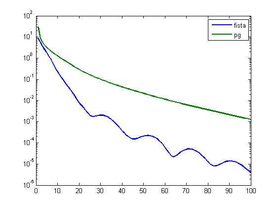

The resulting plot is

Example 2:

In this example we consider the problem

$\|A(x)-b\|_F^2+\lambda \|W(x)|_1$

where A represents a blurring operator with a Gaussian PSF and W is an orthogonal wavelet transform. b is the observed image. The l₁ norm on W(x) is the natural extension of the l₁ norm on vectors, meaning that it stands for the sum of absolute values of the components of W(x) (it is not the induced l₁ matrix norm).

We begin by generating the "true" image, which in this case will be the cameraman.

>> X = double(imread ('cameraman.pgm') );

>> X = X/255;

Next we construct the a Gaussian PSF that will be used in the blurring operator A

>> [P,center] = psfGauss([9,9],4)

The function psfGauss was taken from the HNO library written by Per Christian Hansen, James G. Nagy, and Dianne P. O'Leary for the book "Deblurring Images: Matrices, Spectra and Filtering". The observed image is produced by blurring X followed by the addition of some noise.

>> B = imfilter(X,P,'symmetric') ;

>> randn('seed',314);

>> Bobs = B + 1e-3*randn(size(B));

We can plot the "true" and "observed" images.

>> figure(1)

>> subplot(1,2,1)

>> imshow(X,[]);

>> subplot(1,2,2);

>> imshow(Bobs,[]);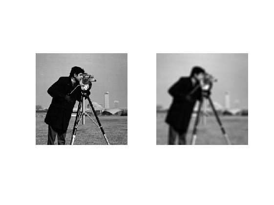

We will solve the deblurring problem using FISTA with

$f(x)=\|A(x)-b\|_F^2, g(x) = \|W(x)\|_1, \lambda =0.001$

The function handles for the objective function and its gradient are

>> fpic = @(x) norm(imfilter(x,P,'symmetric') - Bobs,'fro')^2;

>> grad_fpic = @(x) 2* imfilter(imfilter(x,P,'symmetric')-Bobs,P,'symmetric');

The wavelet transform used in this example is taken from the "numerical tours of signal processing" written by Gebriel Peyre that can be downloaded from the MATLAB's file exchange website.

>> options.ti=0;

>> Jmin=4;

>> w= @(f) perform_wavelet_transf(f,Jmin,+1,options);

>> wi= @(f) perform_wavelet_transf(f,Jmin,-1,options);

The function g and its prox mapping are implemented next.

>> Gpic = @(x) sum(sum(abs(w(x))));

>> prox_gpic = @(x,a) wi(prox_l1(w(x),a));

In the above we used the fact that since W is an orthogonal transformation, it holds that

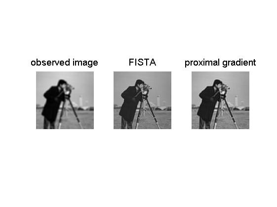
${\rm prox}_{\alpha g}(x) = W^T(\mathcal{T}_{\alpha}(W(x)))\quad \forall \alpha>0$

We now run 100 iterations of FISTA and the proximal gradient method. The image produced by FISTA is significantly better than the one generated by the proximal gradient method.

>> clear par

>> par.max_iter = 100;

>> x_fista= fista(@(x)fpic(x),@(x) grad_fpic(x), @(x) Gpic(x), @(x,alpha)prox_gpic(x,alpha),0.001,zeros(size(Bobs)),par);

>> x_pg=prox_gradient(@(x)fpic(x),@(x) grad_fpic(x), @(x) Gpic(x), @(x,alpha)prox_gpic(x,alpha),0.001,zeros(size(Bobs)),par);

>> figure(2)

>> subplot(1,3,1)

>> imshow(Bobs,[])

>> title('observed image','FontSize',14)

>> subplot(1,3,2)

>> imshow(x_fista,[])

>> title('FISTA','FontSize',14)

>> subplot(1,3,3)

>> imshow(x_pg,[])

>> title('proximal gradient','FontSize',14)

*********************

FISTA

*********************

#iter fun. val. L val.

1 62.790523 2.000000

2 23.292874 2.000000

3 12.229700 2.000000

4 8.239808 2.000000

: : :

97 3.040138 2.000000

98 3.039991 2.000000

99 3.039849 2.000000

100 3.039708 2.000000

----------------------------------

Optimal value = 3.039708

*********************

prox_gradient

*********************

#iter fun. val. L val.

1 17380.441112 2.000000

2 62.790523 2.000000

3 23.292874 2.000000

4 13.973323 2.000000

: : :

96 3.262200 2.000000

97 3.259289 2.000000

98 3.256438 2.000000

99 3.253645 2.000000

100 3.250909 2.000000

----------------------------------

Optimal value = 3.248227

Obviously, the image produced by FISTA is better than the one generated by the proximal gradient. This is also reflected by the obtained function values (3.039708 for the FISTA and 3.248227 for the proximal gradient method).

Example 3:

Consider the problem

$\min_{x \in {\mathbb R}^3} \sqrt{1+\|Ax\|_2^2}+\|Bx+b\|_2$

where

>> A=[1,2,0;2,1,2;0,2,1];

>> B=[1,0,-1;2,1,3];

>> b=[1;-1];

We will solve the problem using FISTA by taking

$f(x)= \sqrt{1+\|Ax\|_2^2}, g(x)=\|Bx+b\|_2,\lambda=1$

In MATLAB,

>> f=@(x)norm([1;A*x]);

>> f_grad=@(x)A'*(A*x)/norm([1;A*x]);

>> binv=B\b;

>> g=@(x)norm(B*x+b);

>> prox_g=@(x,a)prox_norm2_linear(x+binv,B,a)-binv;

Running FISTA on the problem yields

>> [out,fmin,parout]=fista(f,f_grad,g,prox_g,1,zeros(3,1));

*********************

FISTA

*********************

#iter fun. val. L val.

1 1.311762 2.000000

2 1.289577 8.000000

3 1.284966 8.000000

4 1.284646 8.000000

7 1.284643 8.000000

8 1.284643 8.000000

10 1.284643 8.000000

11 1.284643 8.000000

Stopping because the norm of the difference between consecutive iterates is too small

----------------------------------

Optimal value = 1.284643

Note that the overall number of iterations is 13 (the last displayed iteration number is 11 since the function value did not improve in the last two iterations).

>> parout.iterNum

ans =

13

Note that the method stopped before it reached the maximum number of iterations (default=1000) since the distance between the last two consecutive iterate vectors was smaller than the default of par.eps (1e-5). We can tighten this parameter to 1e-7.

>> par.eps=1e-7

>> [out,fmin,parout]=fista(f,f_grad,g,prox_g,1,zeros(3,1),par);

*********************

FISTA

*********************

#iter fun. val. L val.

1 1.311762 2.000000

2 1.289577 8.000000

3 1.284966 8.000000

4 1.284646 8.000000

7 1.284643 8.000000

8 1.284643 8.000000

10 1.284643 8.000000

11 1.284643 8.000000

15 1.284643 8.000000

18 1.284643 8.000000

Stopping because the norm of the difference between consecutive iterates is too small

----------------------------------

Optimal value = 1.284643

>> parout.iterNum

ans =

20

This time the method stopped after 20 iterations. If we want to enforce the method to employ the default of 1000 iterations, then we can set par.eps to 0.

>> par.eps=0

>> [out,fmin,parout]=fista(f,f_grad,g,prox_g,1,zeros(3,1),par);

*********************

FISTA

*********************

#iter fun. val. L val.

1 1.311762 2.000000

2 1.289577 8.000000

3 1.284966 8.000000

4 1.284646 8.000000

7 1.284643 8.000000

8 1.284643 8.000000

10 1.284643 8.000000

11 1.284643 8.000000

15 1.284643 8.000000

18 1.284643 8.000000

21 1.284643 8.000000

22 1.284643 8.000000

25 1.284643 8.000000

26 1.284643 8.000000

28 1.284643 8.000000

29 1.284643 8.000000

31 1.284643 8.000000

----------------------------------

Optimal value = 1.284643

>> parout.iterNum

ans =

1000

Note that no function value is printed after iteration 31 since the objective function value was not improved (although 1000 iterations were employed).