Interferometry

Theoretical Background

Diffraction and Interferometry

Light is a transverse wave described by the equation "E(x,t)=A₁cos(kx-ωt)" where E is the electric field, A₁ is the amplitude, ω is the wave's frequency, k=2π/λ is the wavenumber, t is time and x is the distance traveled. Suppose two waves differing only by a phase φ meet: E₁ + E₂ = ... . We get a new wave multiplied by cos²(φ/2). In the case of φ = π, 3π, 5π etc When two waves of same wavelength and polariztion travel through the same medium, their amplitudes combine. A wave of greater or lesser amplitude than the original will be the result. The addition of amplitudes due to superposition of two waves is called interference. When both phases roughly match, the amplitudes are added together and the result will be of higher intensity than the sum of the original two and this is called contructive interference. Conversly, when the phases are roughly opposite to one another (the difference is roughly π), in the specific case when the two waves have the same amplitude as well, the maximum of one wave meets exactly with the minimum of the other. The resultant intensity will be zero and the waves are said to interfere destructively.

A light wave can be described by its frequency, amplitude, and phase, and the resulting interference pattern between two waves depends on these properties, among others. The two-beam interference equation for monochromatic waves is:

where I₁,I₂ are the intensities of the original waves, which are the electric field amplitudes A₁,A₂ squared (I∝A²). φ is the phase of the wave, but what actually matters is the relative phase between the waves: Δφ=φ₁-φ₂.

When Δφ is an integer of 2π, the resulted intensity will be maximal. Note that in the specific case of equal intensities (I₁=I₂=I):

When Δφ is an odd integer of π, the resulted intensity will be minimal and in the specific case of equal intensities:

Note that if the initial intensities of the arms aren’t equal it is impossible to achieve complete destructive or constructive interferences.

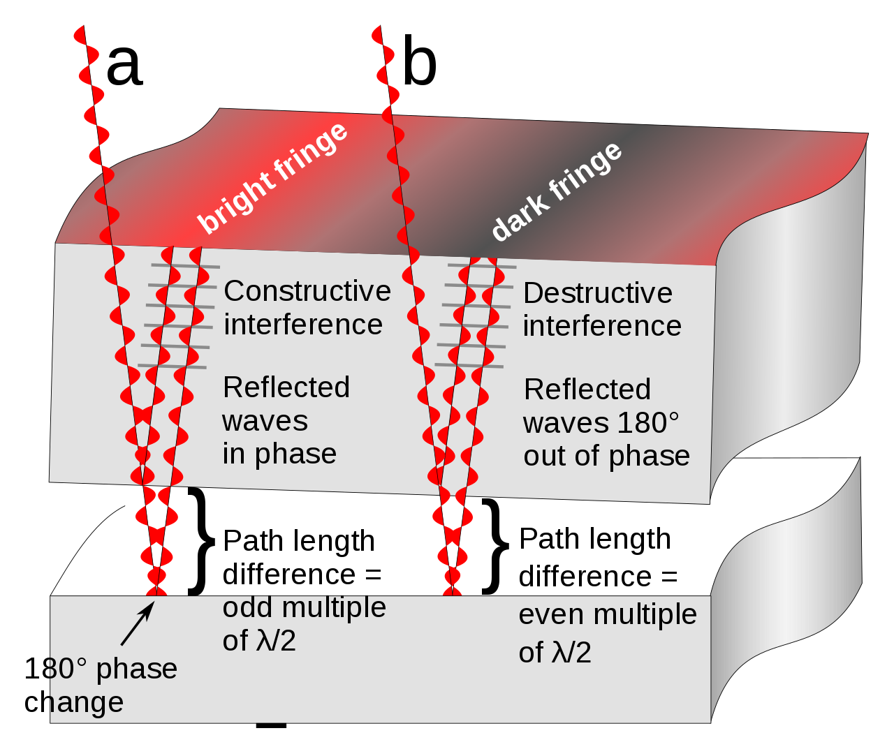
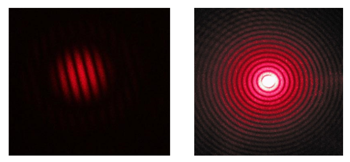
A reflector adds a π phase shift to the waves. Therefore, in the figure above, if the arms are initially separated by path difference of an odd multiple of λ/2 (a), the phase shift will sum up to a multiple of 2π and the two reflected beams will be perfectly aligned at their crests and troughs. In the case of a path difference of an even multiple of λ/2 (b), the phase shift will sum up to an odd multiple of π, and the two reflected beams will be perfectly aligned crest to trough and vice versa. An important note: A slight tilt of the reflector will not change the optical path, yet it will cause a periodical structure of these path differences, manifested in an interference pattern of light-dark-light lines, as shown in the next figure on the left. This ineterference pattern will allow us to study and understand this unique phenomenon - spatial interference.

For a monochromatic light source with a wavelength of λ, the number of cycle transitions in the interference pattern, N, can teach us about the separation between the two arms:

where l is the optical path difference of the beams in the interferometer. The factor of ½ is added since every movement of the translation stage by Δx, from which one of the arms is reflected, doubles the path difference to 2Δx. Having a known path difference, l, allows extraction of the source’s wavelength by calculation of number of cycles.

Michelson Interferometer

The Michelson interferometer is the best example of what is called an amplitude-splitting interferometer. It was developed by Albert Michelson, and used in 1893 to measure a standard meter in units of the wavelength of the red line of the cadmium spectrum. With an optical interferometer, one can measure distances directly in terms of wavelength of light used, by counting the interference fringes that move when one or the other of two mirrors are moved. In the Michelson interferometer, coherent beams are obtained by splitting a beam of light that originates from a single source with a partially reflecting mirror called a beam splitter. The resulting reflected and transmitted beams are then re-directed by ordinary mirrors to a screen where they superimpose to create fringes. This interferometer, used in 1887 in the famous Michelson-Morley experiment, demonstrated the non-existence of an electromagnetic-wave-carrying aether, thus paving the way for the theory of Special Relativity.

A simplified diagram of a Michelson interferometer is shown in Figure 3:

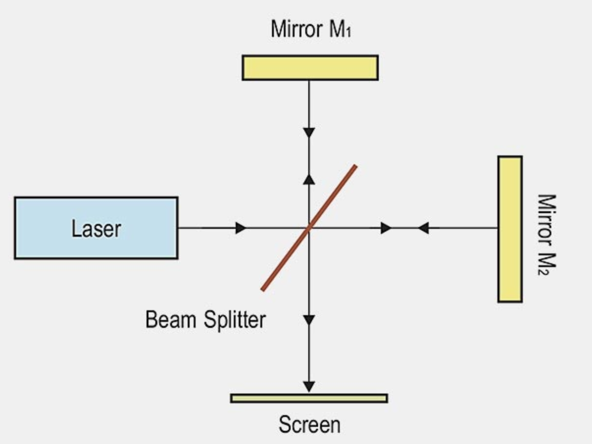
Light from a monochromatic source is divided by a beam splitter, which is oriented at an angle 45° to the beam, producing two beams of equal intensity. The reflected beam travels to mirror M₁, where it is reflected back to the beam splitter. 50% of this beam is transmitted straight through and reaches the screen- eventually, 25% of the initial output intensity. The transmitted beam travels to mirror M₂ and it is reflected back to the beam splitter. 50% of the returning beam is then reflected by the beam splitter and strikes the screen (also with 25% of the initial output intensity).

Mach-Zehnder Interferometer

This interferometer was first developed by Ludwig Zehnder in 1891, and slightly refined by Ludwig Mach in an 1892 article. Unlike the Michelson interferometer, each of the separated light paths in the Mach-Zehnder configuration is traversed only once, making it a highly configurable instrument.

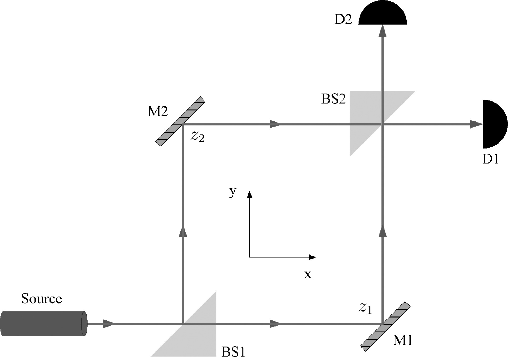
BS1 and BS2 represent beam splitters, M1 and M2 represent mirrors, and D1 and D2 represent detectors. Each reflection (from a beam splitter or mirror) introduces a π phase shift to the electromagnetic wave. The difference in optical paths, which can be due to a difference in distance travelled or by introduction of something into one of the interferometer arms, determines the output at the detectors.

The main difference between the two types of interferometers is that while the Michelson version has a single output, the Mach-Zehnder version has two outputs that complement each other with an appropriate π phase shift (read more about it in the following paper). If the optical paths for both interferometer arms are equal, we will have a fully constructive interference in one detector (intact spot of light), and a fully destructive interference in the other detector (complete darkness). Practically speaking this is very hard to obtain, as there will always be some difference in path lengths due to finite accuracy in the optics and their positioning and alignment. However, there will always be a π phase shift between the two detectors, i.e. we will always see on one detector the complementary part of the interference observable on the other detector.

An important note: an interference of the two arms will be observable as long as the path difference between the arms is shorter than the source's coherence length.

Refractive Index of a Medium

The refractive index of a medium, n, determines the speed, in which light travels through it:

where v is the velocity of light in the medium and c is the speed of light in vacuum. The maximal light velocity is c; therefore, n is always a dimensionless number larger than 1 (or equal to 1).

The refractive index also determines the degree of refraction of light when it travels through a medium:

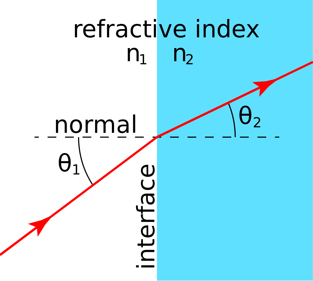
A beam traveling through a medium with the index n₁, with the relative (to the normal to the media interface) angle θ₁ will be refracted at the second medium with n₂ by the angle θ₂. According to Snell’s law, the relation between the angles is as following:

Consequently, when a light beam propagates perpendicularly to the interface and thus θ₁ is exactly 0°, there will be no refraction by the second medium.

In an interferometer setup we have the ability to measure exactly how a sample delays the light propagation inside it, by comparing its path to the course of the second beam. If before placing the sample the paths of both arms were equal, we can now express their path difference only by properties of the sample. Let us start with the simple case, where the sample is perpendicular to the beam. The beam will pass through the sample with velocity v and by time t it will propagate a distance that is equal to the sample thickness, d.

By that time, the second arm will propagate a distance, x with the speed of light:

What we are interested in is the path difference between the arms, i.e. the difference l=x-d:

where Δn is the difference between the refractive index of the sample and the index in air (=1). The path difference is manifested in the number of observed fringes, multiplied by the beam’s wavelength: (Since in a Mach-Zehnder interferometer, the light passes through the medium only once, there is no need to divide by 2):

A direct measurement of the interference pattern enables us to extract the index of refraction of a sample with a known thickness, d:

However, this direct measurement is practically impossible, since the changes in the diffraction pattern are very rapid when inserting the sample and the quantification of N is not feasible. Therefore, the extraction of the refractive index must be performed by rotating the sample and counting the interference fringes during the rotation.When the sample is rotated by an angle of θ towards the wave front of the beam, we need to observe the following scheme:

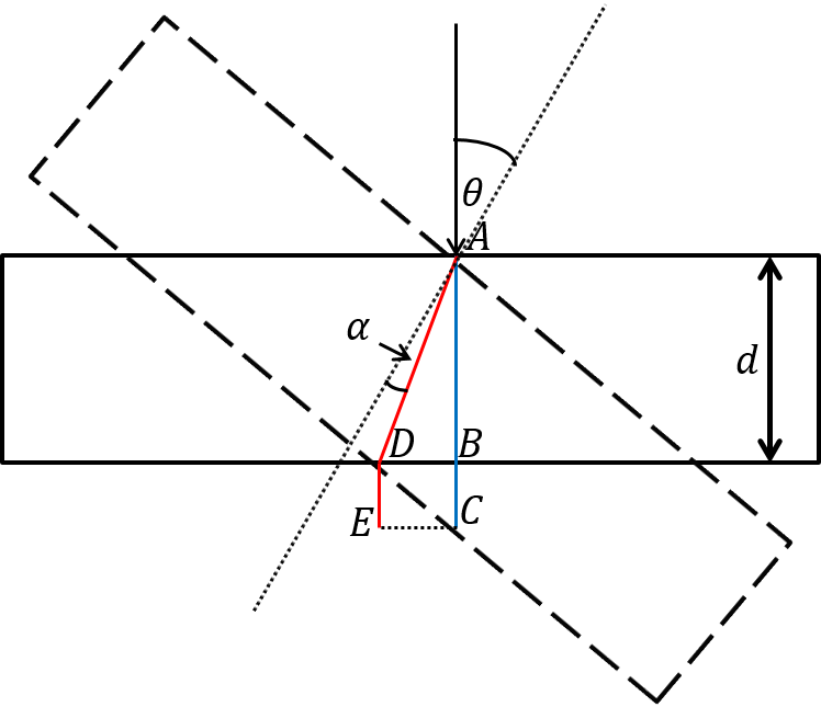
The tilt of the sample by an angle of θ causes refraction of the beam in the medium, by an angle of α. An elongation of its path from AC to AE occurs. The total optical path between A and C initially is: n∙d+BC. When the sample is rotated the optical angle is increased to AD∙n+DE.The total increase in optical path of light propagating through a tilted sample, relative to a perpendicular sample is:

Using the geometrical identities:

we can rewrite the expression:

Finally, using Snell’s law: n·sinα=sinθ, we can extract an equation for the index of refraction, depending on the sample thickness and its angle of rotation:

Note that this expression is correct for the Mach-Zehnder interferometer, where the light passes through the sample only once. For the Michelson configuration, the path difference, l, is twice as long. Since this equation is wavelength dependent, it is irrelevant for our Michelson interferometer experiment. There we will calculate the index of refraction via the modifications in the frequency domain spectrum of the light. Read more about it in the experimental procedure section.

Laser

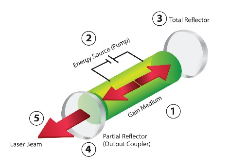
This commonly used term is actually an acronym, LASER, standing for Light Amplification by Stimulated Emission of Radiation. As this name suggests, a laser emits light through stimulated emission of electromagnetic radiation. This is what gives lasers their monochromaticity and coherence, as release of photons from a medium by this mechanism dictates that the photons will have the same phase, frequency and polarization as their pumping source. A laser has an optical cavity – a confined space sealed by mirrors of well-defined positions on opposite sides. This cavity is filled by a gain medium – basically some material that can be put into an excited electronic state by introducing external energy into the system, usually another light source, such as another laser of a different wavelength or an electrical discharge serves as this energy source or pump. This external energy interacts with photons in the cavity, through stimulated emission, to emit more of the same type of photons. To achieve the desired amplification effect, one needs to get population inversion, meaning that more of the medium is in its excited state than in the ground state. Upon population inversion, stimulated emission occurs more frequently than absorption and the number of photons increases. Some of the light then escapes (controllably) through one side of the cavity, usually through a limited aperture - this is the laser radiation. A schematic of the operation of a laser is shown in Figure 7. You can also watch this YouTube video, which illustrates the main concepts of laser operation.

A laser has defining characteristics: wavelength, spectral bandwidth (which also defines coherence), and power. If the laser is pulsed, temporal bandwidth and pulse duration (which influences coherence) are additional important properties. The wavelength of a laser is simply the central point (maximum) of the radiation spectrum emitted from its cavity – defined in meters as is all electromagnetic radiation. The power is the amount of radiation energy emitted per unit time from the laser cavity. The bandwidth of the laser (given either in wavelength or in frequency) is a measure of how accurate the device. In the case of a He-Ne CW (continious wave) laser the bandwidth is very narrow, allowing long temporal coherence and, consequently, a long coherence length.

Thermal Source (Black Body)

Substances that have a finite temperature are thermal sources of light, or electromagnetic radiation. This means that virtually everything emits electromagnetic radiation. Unlike a laser-based source, a thermal source typically has a very wide spectral distribution, meaning it emits light in a broad band of the electromagnetic spectrum. Generally, we can approximate a thermal source as a black-body radiator (i.e. a source for which radiative emission is dependent only on its temperature). The spectral density (in W/m³ units) of such a source can be modeled using Planck's law: $$ \rho (λ,T)={8πhc^2\over λ^5} {1 \over e^{hc/(λk_B T)}-1} $$ where k_B is the Boltzmann constant, h is the Planck constact, c is the speed of light in the medium and T is the temperature. This equation gives the energy density per time per volume in the spectrum. In our experiment, a standard tungsten lamp will serve as a thermal source. Control over its spectrum is achieved by changing the current we run through its tungsten filament.

Coherence Length

The coherence of light is a crucial property for observation of interference fringes and their accurate quantification. The light of one arm must be both spatially and temporally coherent with the other arm. A source can produce fringes as long as the optical path difference between the two beams is less than the coherence length. There are additional conditions to be met for proper interference, such as polarization compatibility of the beams and relatively close intensities.

The temporal coherence of light, translated to its coherence length, is dependent on its bandwidth- the more monochromatic it is, the longer its coherence length. Therefore, a CW (continuous wave) laser, will have larger coherence than a long pulse (of a few picoseconds, for instance) laser, that will have longer coherence length than an ultrashort, femtosecond pulse laser. This is due to the uncertainty principle:

Using the relation E=pc:

The greater the uncertainty of a particle’s energy (or frequency), the smaller its uncertainty in time.

The time-frequency coupling dictates that the narrower the pulse in time is, i.e. the smaller its uncertainty is in time, the wider the pulse’s bandwidth. For example, a laser is often modeled as a purely monochromatic source; that is, its spectral bandwidth is zero. Having a zero frequency bandwidth results in the temporal coherence of a purely monochromatic source being infinite. Infinite temporal coherence means that light of one beam can be delayed relative to the second by any amount of path length, and the two beams will still interfere.

The temporal coherence if light can be quantified both by coherence length, L_c, and coherence time, τ_c:

We can calculate the coherence lengths of the relevant sources for our experiments. For a He-Ne laser with a principle wavelength of λ₀=632.816 nm, the bandwidth in wavelength is Δλ<1 pm:

The meaning of this result is that the He-Ne laser remains temporally coherent and can manifest an interference pattern even if the arms differ in their path by more than 40 centimeters. The coherence time is in the nanosecond regime:

In the case of a tungsten light bulb, the principle wavelength is λ₀=550 nm, but the bandwidth is much larger now, Δλ~300 nm since it is a black-body emission:

Here, the white light source remains temporally coherent for about a micron!

If it is decided to produce fringes with this source, then, because of its limited coherence length, great care must be taken to equalize the optical paths or no fringes will be visible. This is one of the reasons for detecting the interference in a white light source using a spectrometer and not by spatial overlap of the arms. Imagine you have a source with a single frequency and you conduct a simple interference experiment with this source. Now imagine that this frequency drifts over time, meaning that it changes slowly as time passes. If you split the two paths from your source (such as in a Mach-Zehnder interferometer in Figure 4) to a distance long enough, you might not get the same interference as expected. This loss of coherence obscures the interference as the more the fringe contrast decays (making meeting the phase criteria less likely) – the worse the coherence and the lower the interference visibility.

Spectral Interferometry

As shown in the previous section, a white light is a broadband source, therefore the observation of spatial interference (of photons in each of the frequencies) is practically impossible. Additionally, the broad bandwidth results in a very short coherence length of the source. A good solution for this obstacle can be observation of the spectral fringes that are generated between the arms. The spectral fringes are the result of the interference (phase difference) of each of the frequencies that the light is consisted of. By analyzing the spectral data, we can calculate the separation between the arms, bypassing the need of a monochromatic light as shown in equation 4, and the very restricted capability of counting interference cycles. In spectral interferometry the spectrometer allows us a highly resolved separation between the different wavelengths and good sensitivity to very slight translations.

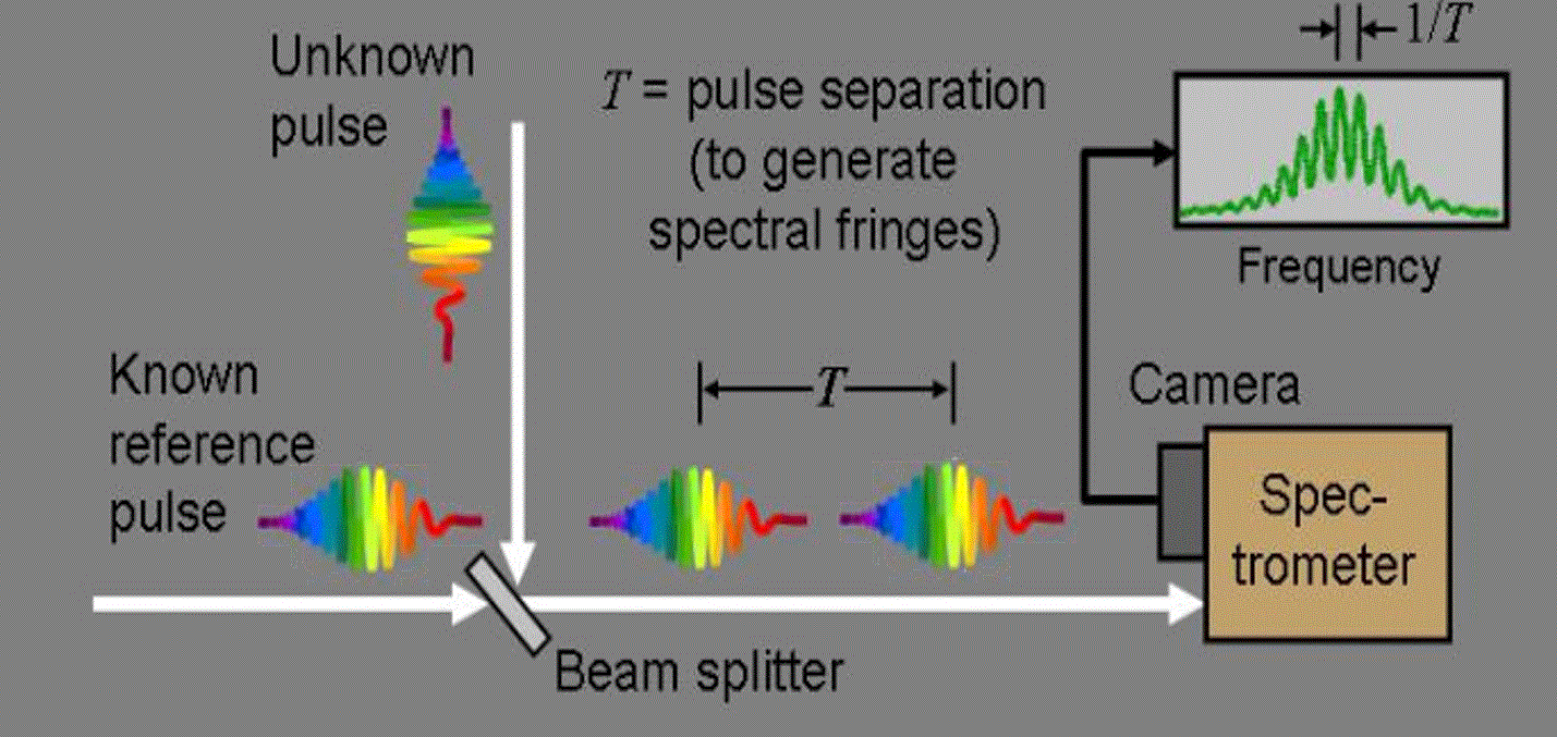
Our thermal source does not generate pulses but the principle is similar. The reference beam is the static, well located arm, while the ‘unknown’ beam is the dynamic arm with a modifiable optical path length. Having a Δt separation between the pulses, the frequency of fringes in the spectrum is proportionate to 1/Δt. In our lab's software the spectrum is given as a function of wavelength, therefore, the fringes you will observe are with varying spacings. It is crucial to change the wavelength axis to a frequency axis, since the relation between them is reciprocal and so is the fringes' spacings:

This spectrometry method allows interferometry with very broadband and incoherent sources. Unlike spatial interferometry, where the resolution is limited by the source’s wavelength (since it is impossible to count less than one fringe cycle), here the resolution is limited by the spectrometer. The spectral resolution dictates the minimal separation between the arms that we can quantify, and it depends on the finesse of the grating that separates the different wavelengths in the spectrometer.

Time-Frequency Relation (Fourier Transform)

A part of your data analysis relies on performing a translation from the frequency domain spectrum to time domain information. This can be achieved either by extracting peaks from the frequency dependent spectrum and calculating the intervals between them, or by applying a Fourier Transform on this spectrum. The Fourier transform is a mathematical calculation, that represents a function in one domain, usually referred to as the time domain, in a second domain, usually referred to as the frequency domain. Fourier transform can be applied for transitions between any coupled domains such as t↔ω, x↔k, that have reciprocal physical units. It is most useful when working with periodical functions, since they will have an elegant representation in the frequency domain, consisted of a finite and discrete number of frequencies. The mathematical expression of the Fourier transform is an integral (Note that the following demonstrations are for an angular distribution, ω=2πν):

For example, if the time dependent function we wish to transform is a sine: g(t)=Asin⁡(ω₀t), its Fourier transform will yield a two peak delta function at the frequencies ±ω₀:

When working with a pulse, i.e. an electromagnetic field multiplied by a Gaussian envelope, its Fourier transform will yield a Gaussian in the frequency domain. The relation between the pulse duration in time (the Gaussian’s variance, manifested in its FWHM) and its bandwidth- the FWHM of the Gaussian in the frequency domain can be extracted by the Fourier transform calculation:

For simplicity, let’s assume t₀=0:

After some math, the solution for each integral is given by a Gaussian:

We got two Gaussians, with central frequencies of ±ω₀. From this result we learn that if the variance of the time-domain Gaussian is σ², it is exactly 1/σ² in the frequency domain. (Relation between FWHM and variance: FWHM=2√ 2ln2 σ)

For example, the simulated pulse below is of FWHM=1 ps duration, and a central frequency ω₀=5 THz=5•10¹² Hz: (t₀=5 ps)

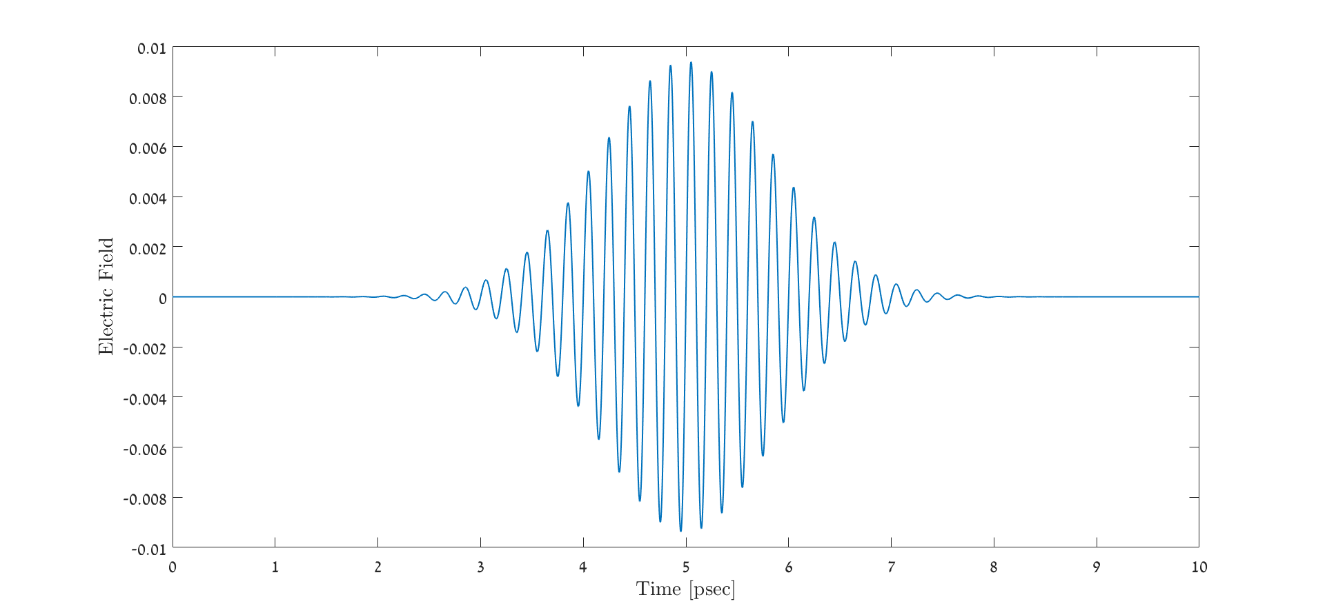
The result of this pulse’s Fourier transform (observing only positive frequencies), is the following Gaussian:

Indeed, we got a single Gaussian, with peak intensity at the frequency of 5 THz, which is exactly ω₀. From a simple fit to a Gaussian function we can extract the variance in frequency domain: σ_ω²=1.506•10²⁴ Hz². Therefore, the FWHM of the frequency domain Gaussian is:

The bandwidth of a 1 psec pulse is of approximately 1.44 THz.

Quantum Mechanics and Interferometry

So far we have observed the light classically, represented as an electromagnetic wave with phase and amplitude. But light can be also described as a quanta of particles called photons. Let us look at a problem involving a single particle, a photon, that can go to through one of two states |A⟩ or |B⟩. When a property of the photon is measured, the result of |A⟩ is a and the result of |B⟩ is b. Now assume that the physical state of the photon is a superposition of these two states:

where α,β∈ℂ. If we measure a property of our photon, one might assume the result will be something between a and b, but this is not the case. The measurement will always yield either a or b, with no absolute certainty of either but never something in-between. This means determinism is lost but the possibilities are well-defined. What can be measured is the probability of each of the states, determined basically by the factors α and β, which can be inferred by repeated measurement to determine the number of times we get a and the number of times we get b. The probability of getting a is proportional to |α|² and the probability of getting b is proportional to |β|². If a and b are the only possible outcomes, and considering conservation of probability (the sum of all probabilities has to be unity) we can write the probabilities:

Note that every time we measure the result a, the state has to become |ψ⟩=|A⟩; and a similar expression can be written for measurement of b. This concept, although algebraically simple, is not at all trivial, as it defies our intuition. The other important, and rather counter-intuitive principle we must take into account to understand our experiment is that interference takes place between every quantum object (or particle) and itself. So for example if we shine light onto two slits (as in Young's experiment), we will get the same result if we pass many photons at the same time, or hurdle them through the slits one after the other as each photon interferes only with itself. This peculiar phenomenon can be related to something more familiar– conservation of energy. If photons were to interfere with other photons, it would have to be possible that two photons with the same amplitude and opposite phase could collide, with the result that all of their energy would disappear. The same goes for in-phase interference – If a photon could interfere with another, a collision of two photons could result in twice the amplitude (i.e. four times the intensity). This is, of course, not a valid physical explanation. The important point to remember is, that a quantum particle interferes only with itself and not with other quantum particles.

Instruments for measurement of optical interference of photons are interferometers. The principle of them is that a quantum object is split into two paths (arms) and recombined before being measured and the output is observed. This is a practical realisation of the experiment described above. Interference of the two states (the particle traversing each arm) can be measured at the interferometer output. This interference is affected by the differences between the two arms. For example, if one arm of the interferometer is longer than the other, particles from both arms will interfere with different phases to create different patterns. The interference pattern obtained contains information about the difference between the paths.