In this experiment you will study photon interference using a Mach-Zehnder and a Michelson interferometer.
Experimental Procedure
Monochromatic Interference (With a Laser Source and Mach-Zehnder Interferometer)
Introduction to Interferometry
Make sure you recognize all of the components in the experimental setups.
Check that the beam paths from the laser and the thermal source are clear to both outputs of the interferometer.
Ensure your surroundings are clear such that the laser light will not harm others working in your vicinity.
Turn on the laser and check the output on the screens.
Check to see if the laser light reaches the screen. Is the beam profile what you expected? You can adjust the beam position by slight changes of the knobs of the last mirrors before the second beam splitter. Ask your instructor before doing so.
Think of a simple experiment that can confirm the energy conservation law by measuring the intensity of light in different configurations of the beams.
Measure the Wavelength of the Laser Source
In this experiment, you will use the interferometer to extract the wavelength of the laser source. Since this is a quantity we know, this measurement will allow you to estimate how well you can control the experimental setup and will allow you to determine what kind of statistics are needed in subsequent experiments.
Record the patterns observed on the screen using the cameras controlled by the laptop. Can you learn anything from these patterns? Discuss your observations.
Record the position of the translation stage.
Begin translating the stage and observe the change in the output on the screen. What do you see? What is happening and why?
Repeat the same action, slowly, and count the number of interference cycles (light-dark-light transitions) as the pattern on the screen changes from light to dark.
Repeat several times for different translation distances. Make sure you record the number of cycles you count.
Determine the wavelength of the laser by plugging in your results into the following formula $$ λ={2Δx \over N} $$ where N is the number of cycles and Δx is the total translation of the stage (factor of 2 is added due to the optical path of the beam, both entering and exiting the stage. Therfore, the translation is double than measured.), and extract the wavelength of the laser, λ.
Measure of the Index of Refraction of a Sample
Similarly to measuring the wavelength of our laser, we can determine the index of refrection or thickness of a sample that is inserted into the interferometer, by measuring the change in the effective optical path that our photons travel in one of the arms of the interferometer. If the thickness of a sample is known, we can extract its index of refraction (or vice versa).
Insert a glass slide in the sample holder in one of the arms of the interferometer. Make sure it is stable.
Rotate the sample holder so that its surface is perpendicular to the beam. You can keep track of the changes in the pattern of the fringes for accuracy: when rotating the sample away from θ=0° (perpendicular), the diffraction pattern changes with the same direction both when rotating to θ or –θ. This means that if your initial θi≠0° , an increase of θ will exhibit a certain trend in the diffraction, while decrease of θ (θ→0) will exhibit the opposite trend.
Once the sample is properly positioned, record the angle of the holder- γi. This is the calibration point, θ=0°. Is it possible to determine the refractive index at this stage (given the thickness of the slide)?
Determine the number of interference cycles (light-dark-light transitions), N, to count on the screen. Rotate the sample holder such that you reach N cycles and record the new angle, γf. (θ=γf-γi).
Extract the refractive index using the following formula: $$ n={({Nλ\over t}+\cosθ-1)^2+\sin^2θ \over 2(-{Nλ \over t} -\cosθ + 1)} $$ where N is the number of cycles, t is the sample thickness, λ is the wavelength of the laser and θ is the rotation angle of the sample.
In order to evaluate the measurement error, you can either repeat the experiment a few times with the same number of cycles or perform it with a few different values of N (and consequently, θ).
Evaluate the Thickness of a Sample With a Known Refractive Index
Repeat the experiment described in section 1.3. using a glass slide of an unknown thickness.
Calculate the thickness of the sample using the refractive index you determined in steps 5,6 from section 1.3. You can extract the sample thickness from the abovementioned equation, after some math: $$ t={Nλ \over {1-\cosθ+\sqrt{n^2-\sin^2θ}-n}} $$
Repeat the previous step using the refractive index from the literature.
Compare your results with a direct thickness measurement. What is the deviation from it? Try to evaluate the range of the possible calculated results from the various error factors.
Witness the Quantum Eraser Effect
The following part will be peformed with the presence of your instructor.
Align the laser beams to produce an interference pattern. Record the patterns on the screens.
Introduce a linear polarizer to one of the interferometer arms. What happens? Record the patterns.
Move the polarizer to the other arm. What has changed?
Introduce a second linear polarizer to the interferometer (one polarizer in each arm), which is perpendicularly polarized to the first one, and a quarter-wave plate at the output of the laser.
Record the patterns on the screen. What is the reason for the effect you are seeing? What would happen without the quarter-wave plate?
Introduce a third linear polarizer at one of the outputs of the interferometer (after the second beam splitter) and note the change.
Rotate the third polarizer and record the change. Make sure you make at least one full 360 degree turn. Note the eight special positions in the cycle of the polarizer. Record them and explain what is happening.
White Light Interferometry (using a Michelson Interferometer)
Quantify the Optical Path Difference of the Arms
Take a dark measurement with the specrometer - Sd button in the software.
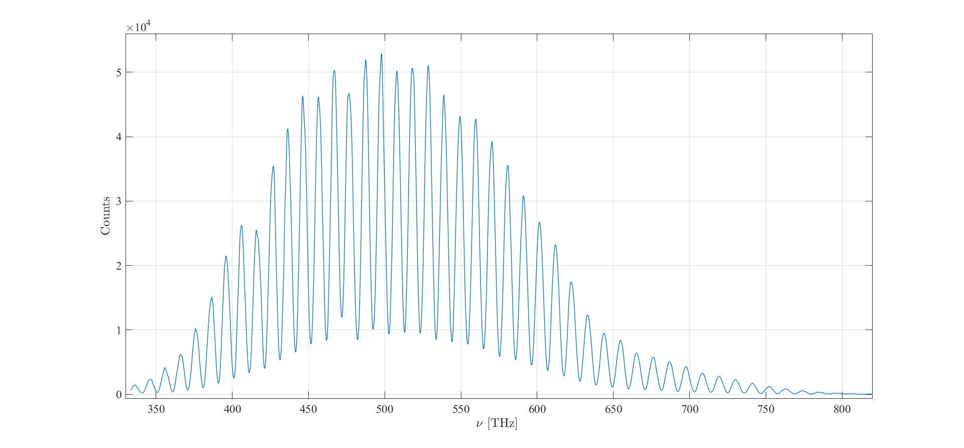
Switch the thermal source on. Turn on the power such that the intensity of the light is enough for you to easily observe the spectrum (around 50,000 counts in the software). An example of the observed spectrum with an interference pattern:
If what you see on the screen does not resemble this example, consult your instructor.
Once you achieved the “comb” pattern, export the data to an Excel file.
In order to quantify the Δx difference between optical paths, process the data you have exported:
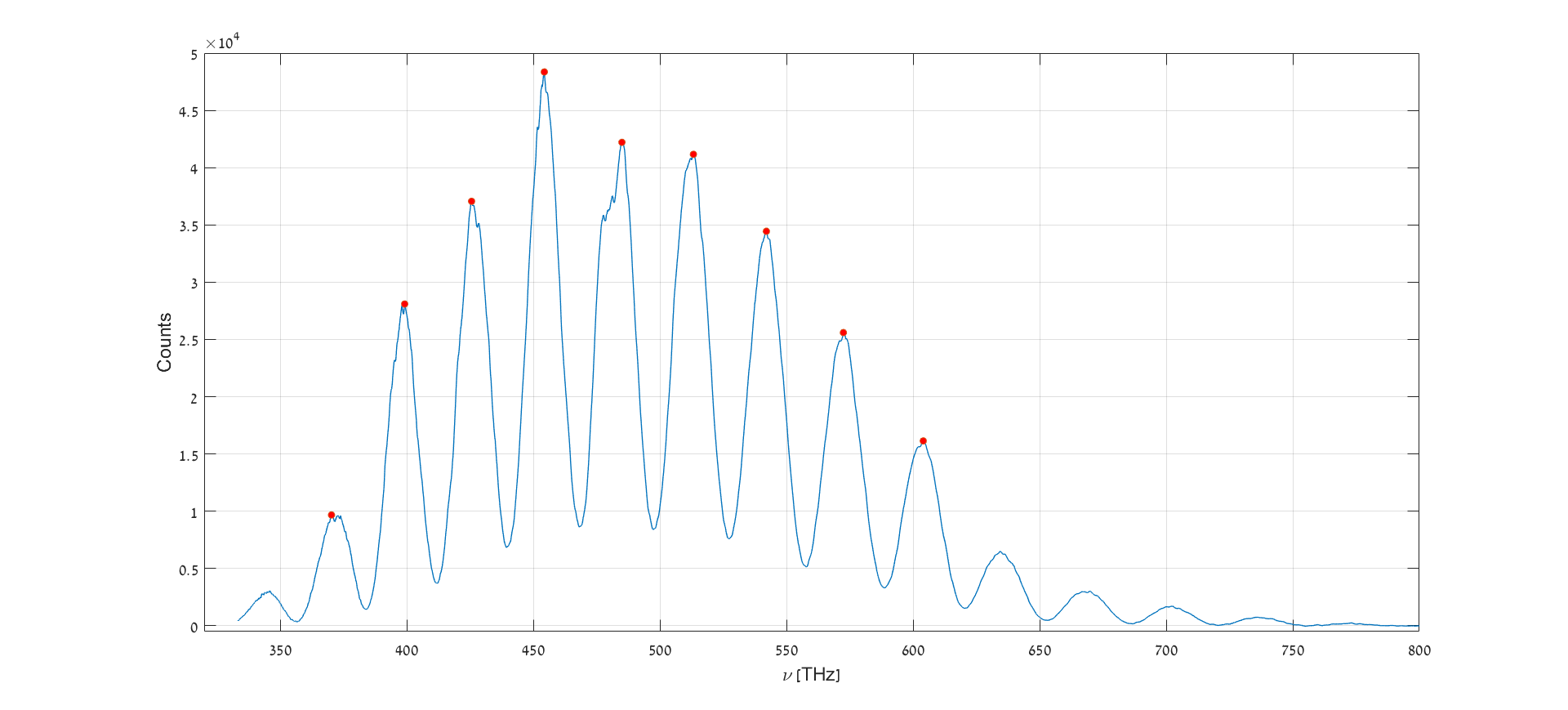
First, you are required to convert the x axis from wavelength to frequency according to the relation ν=c/λ. Now, you can observe the signal intensity at each frequency. This is the converted frequency comb of the spectrum above:
Note that the spacing between the peaks is now roughly constant, while in the original data it changed with the wavelength. Why?
You can either count and locate the peaks manually, or use the Matlab online software, and the "findpeaks" library function.
A suggested syntax:
[pks, locs] = findpeaks (signal, 'MinPeakHeight', n, 'MinPeakDistance', m);
For the vector “signal”, the function extracts the values (pks) and indices (locs) of all peaks that are above the threshold value n, with minimal spacing between them of m points. The threshold allows us to find only local maxima and not minima and the spacing enables consideration of only one maximum point in a given peak, although isn’t smooth.
Using “locs”, which are the indices of the peaks, you will be able to also extract the frequencies that belong to these peaks, having the same indices. An example of the result of this function are scattered dots in the following frequency comb spectrum:
Calculate the spacing in frequencies, Δν. Make sure it is not frequency dependent.
The average Δν can be translated to an average difference in the timing Δt according to relation Δt=1/Δν (here Δ stands for interval and not uncertainty). Since the speed of light is a known constant, the difference in timing is directly translated to the difference in space by Δx=cΔt.
Quantify the error of Δx. What is the main contributor to this error?
Quantify the Interferometer Translation
Move the stage very slightly in one direction and export the data to a new Excel file. Make sure that you don’t cross the “zero point” (characterized by a very wide doublet spectrum). What happened to the spectrum?
Now repeat step 1 in the opposite direction, crossing the point you were at initially (before step 1), without crossing the “zero point’. Export the data. What happened to the spectrum this time? What is the difference from the previous step?
With the data from part 2.1, you should now have in total three different spectrum data sheets.
Quantify the differences in optical paths, Δx as in part 2.1 for both positions of steps 1 and 2. The total translation, l= Δxf - Δxi where Δxi is the distance you found in part 2.1, and Δxf is the distance you extract for each spectrum in steps 1 and 2.
Intensity Modulation of the Arms
Move the stage carefully in order to achieve a sufficiently dense modulation (difference between maximal and minimal signals) pattern on the screen, so that:
You can approximate that a local maximum and minimum are practically at the same wavelength.
You can assume that the original intensity of the spectrum (of one of the arms) is approximately constant.
Consult with your instructor before saving the data.
From this data you can calculate the experimental intensity modulation:
$$ M_{exp}= {I_{maximal} \over I_{minimal}} $$
Block one of the arms and save the spectrum.
Repeat step 3 for the second arm.
Calculate the theoretical intensity modulation from the measured data in steps 3,4 according to following equation and compare your experimental result:
$$ M_{theory}= {{(\sqrt{I_1} +\sqrt {I_2} )^2} \over { (\sqrt {I_1} - \sqrt {I_2} )^2}} $$
where Mtheory is the theoretical modulation and I1,I2 are the intensities of each of the arms. Note that the interference occurs between the electric fields and not intensities, therefore the calculation of square root of each intensity is required.
Demonstrate the Law of Energy Conservation
Before beginning this part, refer to your instructor for guidence regarding the optical alignment of the setup.
Place an additional beam splitting cube before the original beam splitter. Make sure that:
The reflection from it is in the correct direction (the writing on the cube should be facing toward you).
The incident beam does not pass thorugh this beam splitter before it is reflected from the first mirror in the optical path.
The incident beam is not cut by this beam splitter. If it is, the beam diameter should be modified with the iris diaphragm near the source output.
The reflection from this beam splitter is aligned, and passes through a lens that is placed at the end of the path (in order to focus the beam into the optical fiber). Since it is very weak, you may need to dim the lights in the lab and turm off the computer screen to be able to see this beam.
Now only half of the intensity is transmitted to the original beam splitter and creates the interference pattern of the spectrum.
You now need to optimize the interfernce pattern you see on the screen, since the beam propogates through this additional cube, and the two arms do not prefectly overlap after this modification.
Export the data to an Excel file (this is interference pattern #1).
Move the (red) optical fiber to the output from the new beam splitter and optimize its position according to the spectrum on the screen (you will need to optimize the beam incidence into the fiber with the last mirror before the lens). Do you expect to see the same spectrum with the same intensities as before?
Export this data to an Excel file (this is interference pattern #2).
Display this data in the same graph with the data from step 3. Discuss your observations in both axes- wavelength and intensity. How what you see is indeed verification of energy conservation?
Measure the Index of Refraction of a Solid Sample
In this part you will insert a sample in the sample holder in the constant arm of the interferometer.
First, remove the beam splitting cube you have inserted in the previous part, and return the optical fiber to its original position. Optimize the interfernce pattern you see on the screen now.
In order to be able to measure the refractive index of the sample you must first move carefully the stage to a position where the addition of this thin sample will:
Not completely destroy the interference (characterized by a normal ‘black body radiation’ spectrum). In this case we will not be able to extract any data about the sample.
Not cross the “zero point” in the translating arm, because then we will not be able to determine the refractive index correctly. Think of the following example: Initially the translating arm is longer than the constant arm by exactly Δx=-90μm (minus for when the arm with the sample holder is shorter than the other arm). By adding a 180 μm thick glass slide (n=1.5) to the constant arm we are extending this arm's optical path by l=Δn•2d=180μm (Δn is the diffrence between the refractive index of the sample and of air, d is the thickness of the sample. Since in a Michelson interferometer the light passes through the medium twice, a factor of 2 is added). But because the translating arm was the longer arm we must cross the “zero point” and we will end up with the same Δx=90μm, and the same initial spectrum! The sign of Δx does not change the spectrum. Make sure you understand why. Actually in this case one can mistakenly think that Δn=0.
After carefully moving the stage to a desirable position, save the spectrum data.This will be your reference position, Δxi.
Only now you can insert the 180 μm sample in the sample holder in the constant arm of the interferometer. Make sure θ≈0° and that the holder is stable. Save the spectrum data. Unlike the Mach-Zehnder interferometer setup, you can extract the refractive index without rotating the sample. Why?
Extract the refractive index: first extract Δxf from the data in a similar manner as in part 2.2. Secondly, remember that here the optical path difference is extended by: l=Δxf - Δxi=Δn•2d and not by the translation of the stage.
Measure the Index of Refraction Dependence on the Concentration of a Solution
Measure 25gr of sucrose and dissolve it in 100ml of distilled water. Make sure that you know how to calculate the concentration of this solution.
Insert two empty and clean glass cuvettes – one in each arm. Make sure to not leave your finger prints on it. Why? Make sure θ≈0° in both arms and that the holders are stable.
Fill the cuvette in one of the arms with distilled water. Make sure there are no bubbles in the water. You can use a pipette to diminish the bubbles by pumping and reinserting the water into the cuvette. This cuvette is your reference cuvette and we will not touch it from here on.
The second cuvette should be filled with exactly 2ml of distilled water. Make sure there are no bubbles in the water. This cuvette is the sample cuvette.
Carefully align the interferometer (with the help of your instructor!).
In this part you will extend the reference arm’s optical path of the interferometer by increasing the refractive index of the water solution (by adding a sucrose solution or by adding ethanol). In order to be able to measure the refractive index of the sample you must first move carefully the stage to a desirable position, as was described in part 2.5, step 3.
Only after you achieved a good spectrum (consult your instructor) save the data. This is your reference data.
Add 20-30 μl of the 25% solution to the sample cuvette. Calculate the concentration of the solution in the cuvette. (consider the addition to the volume)
Improve the homogeniety of the new solution using a pipette as in step 3. After reaching optimal homogeniety, the observed spectrum is achieved from the contribution of the solute. Save this data.
Extract the refractive index of this concentration, as in part 2.5, step 5.
Repeat steps 8-10 with at least five more concentrations: Gradually add a constant volume of the 25% solution and recalculate the concentration and save the spectrum after each addition.
Plot the refractive index as a function of concentration.
Try to explain the observed trend. In case of sucrose solution, you can refer to the following paper, but note that this work was done with monochromatic lasers while you extracted data for a thermal source.
Clean thoroughly the sample cuvette and refill it with 2ml of water.