Chemical Physics

Theoretical background

Introduction

The term vacuum refers to the condition of an enclosed space that is devoid of all gases or other material content. It is not experimentally feasible to achieve a “perfect” vacuum, although it is possible to obtain a vacuum of 10^-6 Torr with a simple laboratory set up and, with more sophisticated techniques, a vacuum of 10^-10 Torr (1.3 x 10^-13 bar or 1.3 x 10^-8 Pa). It is even possible by special techniques to obtain a vacuum of 10^-15 Torr, or about 30 molecules per cubic centimeter.

One Torr, the conventional unit of pressure in vacuum work, is the pressure equivalent to a manometer reading of 1 mm of liquid mercury: 1 Torr = 1 mmHg = 1/760 atm = 1.333 x 10^-3 bar = 133.3 Pa.

For Dewar flasks, metal evaporation apparatus, and most research apparatus, a vacuum of 10^-5 to 10^-6 Torr is sufficient; this is in the "high vacuum" range. A vacuum of 10^-10 Torr is termed an "ultrahigh vacuum". For many routine purposes a "utility vacuum" or "forepump vacuum" of about 10^-3 Torr will suffice, and for vacuum distillations only a "partial vacuum" of the order of 1 to 50 Torr is needed.

Many famous scientists have performed investigations under vacuum conditions. You can find interesting information about the history of vacuum science here and information about terminology and technology here. Most modern day experimental research in physical chemistry is performed with the use of some sort of vacuum system. Organic and inorganic chemists also find use of vacuum systems essential as these researchers often conduct synthetic and kinetic work under controlled or reduced pressures.

Vacuum systems vary widely in their size and complexity depending on the requirements of pumping speed and attainable vacuum. This experiment is designed to illustrate the purposes and uses of the basic components found on a typical vacuum apparatus.

Gas flow in tubes

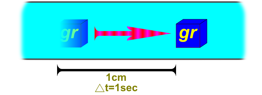
In order to achieve a low pressure in a vacuum line, some air must be removed by pumping. As it is removed, it must flow from one end of the tube to the other. The flow rate of a gas, called the throughput (Q), is defined as:

$$ Q = \frac{d}{dt} PV $$

where P is the pressure at which the throughput is measured, and V is the gas volume.

Notice that throughput does not have the same units as ordinary gas flow rate, which is in unit volume per unit time. The units of throughput are [pressure]·[volume]/[time] or [energy]/[time], that is, L·atm·min^-1(sometimes Torr·L/s, Pa·m³·s^-1 (SI units), J·s^-1, or watts). Thus, they represent power (energy per unit time).

The throughput depends on the resistance to flow and the pressure drop between the entrance and the exit of the tube or channel:

$$Q = \frac{P_2-P_1}{Z} = C(P_2-P_1)$$

where P₁ is the downstream pressure (measured at the exit), P₂ is the upstream pressure (measured at the entrance), Z is the resistance and C is the conductance.

The conductance is the throughput per unit pressure difference between the tube entrance and the exit. The units of conductance are the same as those of volume rate or pumping speed, so conductance can be expressed in L/min, L/s, or m³/hour, for example. In SI units, conductance is measured in m³/s.

Equations (1) and (2) are analogous to Ohm's Law, which relates the flow of current, I, through a resistance R under the influence of a potential difference V as follows:

$$ I = \frac{V}{R}$$

In the case of a vacuum, the equations relate the gas flow, Q,through a tube with resistance Z under the influence of a pressure difference, P₂ – P₁.

Just as the resistance of electrical resistors in series is given by:

$$ R_T = R_1 + R_2 + R_3 + R_4 + \dots $$

and in parallel by:

$$ \frac{1}{R_T} = \frac{1}{R_1} + \frac{1}{R_2} + \frac{1}{R_3} + \dots $$

so the resistance to gas flow is given by:

$$ Z_T = Z_1 + Z_2 + Z_3 + Z_4 + \dots $$

where Z_T is the total resistance, and Z_i are the series resistances of the various components in a vacuum line, that is, the traps, baffles, stopcocks, and tubes of different diameters as shown schematically in Figure 1.

It is somewhat more common in discussing gas flow to speak of conductance rather than resistance, so equation (6) is frequently written:

$$ \frac{1}{C_T} = \frac{1}{C_1} + \frac{1}{C_2} + \frac{1}{C_3} + \dots $$

Series and parallel resistance — Schematic of resistance in series (Z1, Z2 and Z3) and in parallel (at termini).

Different Types of Flow

The nature of gas flow through a tube is quite different at low pressures and at high pressures. In addition, the flow characteristics depend on the flow rate and on the geometry of the tube, pipe, or channel through which the gas flows.

Three kinds of flow are recognized: turbulent, viscous (laminar), and molecular. See a short video illustrating laminar and turbulent flow here.

The Reynolds number, Re, is useful in describing the boundary between turbulent and viscous flow; similarly, the Knudsen number K_n can be used to describe the boundary between viscous and molecular flow. The Reynolds number, which is dimensionless, is defined as:

$$ Re = \frac{a \cdot \rho \cdot U}{\eta} $$

where a is the tube radius, ρ is the gas density, η is the viscosity, and U is the flow velocity across a plane in the tube, defined as:

$$ U = \frac{Q}{\pi \cdot a^2 \cdot P }$$

The Knudsen number, K_n, is purely empirical and is defined as the ratio of the mean free path, L, to a "characteristic dimension" of the system, say, the radius of the tube:

$$ K_n = \frac{L}{a} $$

The Knudsen number is also dimensionless. The mean free path is given by:

$$ L = \frac{1}{ \sqrt{2} \cdot \pi \cdot d^2 \cdot N }$$

where d is the molecular diameter, and N is the number of molecules per volume unit. Since N is related to pressure and temperature, it is convenient to express the mean free path for air at 25 °C as:

$$ L = \frac{0.005}{P} $$

where L is the mean free path in centimeters and P is the pressure in Torr. This provides an estimate of the Knudsen number for a tube or bulb in a vacuum line.

The rough ranges of flow are summarized in Table 1:

Types of gas flow
Flow Type Pressure	Reynolds No.	Knudsen No.
Turbulent High	>2200	-
Viscous Medium	<1200	<0.01
Molecular Low	-	>1.00

As an example, let us calculate the maximum pressure (in Torr) at which molecular flow is observed in a long glass tube of 25 mm in diameter:

$$ L^{min} = K_n^{min} \cdot a = 1.0 \cdot 1.25\text{cm} = 1.25\text{cm} $$

$$ P^{max} = 0.005/L^{min} = 0.005/1.25 = 4·10^{-3} \text{Torr} $$

Viscous Flow Versus Molecular Flow

Above about 10^-3 Torr, gas properties depend upon collisions between molecules, which occur much more frequently than between molecules and their container. At pressures below 10^-3 Torr, collisions between molecules are infrequent so there is no viscosity. In the region of viscous flow, the Poiseuille equation gives the throughput through a straight tube of circular cross section:

$$ Q = \frac{\pi \cdot d^4}{128 \cdot \eta \cdot ℓ} {P_{avg} \cdot (P_2-P_1)} $$

where d and ℓ are the tube diameter and length, respectively, η is the gas viscosity, and P_avg is the average of P₂ and P₁.

If we combine equations (2) and (13), we obtain an equation for the viscous flow conductance in a tube of circular cross section:

$$ C = \frac{\pi \cdot d^4}{128 \cdot \eta \cdot ℓ} P_{avg} $$

Note that the most widely tabulated unit of viscosity is the CGS unit, poise: 1 poise = 1 g·cm^-1·s^-1. The SI unit is 1 Pa·s = 1 kg·m^-1·s^-1. Thus: 1 poise = 0.1 Pa·s (Figure 2).

Poise description — Schematic illustrating the unit poise: 1 poise is the movement of 1 gram a distance of 1 cm in 1 second.

The viscosity of air at 25 °C is: 1.845·10^-4 poise = 1.845·10^-5 Pa·s. If d and l are given in centimeters and P_avg in Torr, then conductance, C, in L/s for air at 25 °C is:

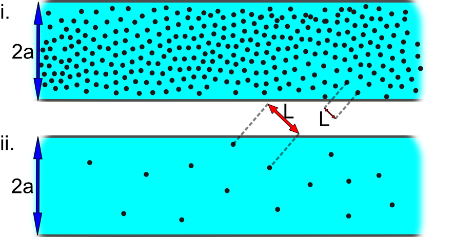
$$ C[L/s] = \frac{d[cm]^4}{ℓ[cm]} 182P_{avg}[\textit{Torr}] $$

Viscous and molecular flow for a mean free path L in a tube of radius a. (i) Viscous flow (L/a < 0.01). The molecules collide much more frequently with each other than with the wall of the containing tube. (ii) Molecular flow (L/a > 1.0). The molecules collide much more frequently with the walls of the containing tube than with each other.

In Figure 3(i), the mean free path (L) is small compared to the radius of the tube (a), and the Knudsen number is L/a < 0.01. In this situation, collisions are more frequent between molecules than they are between molecules and the walls of the container. Consequently, the properties of the gas are quite constant over several mean free paths, and the gas acts like a continuous viscous fluid: The gas flow is considered viscous. In Figure 3(ii), because the mean free path is of the same order (or even larger) than the diameter of the tube (the Knudsen number is L/a > 1.0), the gas molecules collide with the walls of the container more frequently than with each other. Viscosity is then undefined, since there can be no shearing forces between layers of molecules, and no momentum is transferred between molecular layers. These are the conditions for molecular flow.

As you look at the panels of Figure 3, visualize the mean free path in comparison to the dimensions of the tube and to the average distance between molecules.

Pumping Speed in Fixed Pressures

The pumping speed, S, at any point in the vacuum system is defined by the ratio of the throughput Q to the pressure at that point:

$$ S = \frac{Q}{P} $$

The units of S are [volume]/[time], the same as the units of conductance.

In the case of a steady flow (a flow that is not a function of time), the pressure at any point in the vacuum system is constant over time, so equation (16) can be rewritten as:

$$ S = \frac{Q}{P} = \frac{dV}{dt} $$

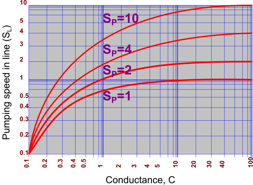
To design a vacuum line properly, it is useful to know how the pumping speed in the line (S_L) differs from the pumping speed of the pump (S_P). The effect of line resistance in reducing the pumping speed is given by:

$$ \frac{1}{S_L}= \frac{1}{S_P} + \frac{1}{C} $$

Notice that if the conductance equals the speed of the pump, the pumping speed in the line is just half of the pumping speed of the pump, since:

$$ \frac{1}{S_L}= \frac{1}{S_P} + \frac{1}{C} = \frac{2}{S_p} \Rightarrow S_L = \frac{S_p}{2} $$

Consequently, it is important to make the conductance of the line as large as possible in comparison to the speed of the pump. It is only when C is infinite (C → ∞ ) that S_L is equal to S_P.

For a real vacuum line, the resistance to pumping is the sum of the resistances of all the components (traps, baffles, stopcocks, etc.) that assemble the line. This relation is usually written in terms of conductances (C = 1/Z):

$$ \frac{1}{S_L}= \frac{1}{S_P} + \sum_{i=1}^{N}\frac{1}{C_i} $$

where the Ci are the conductances of the different components, and N is the number of components. Thus, it is important to minimize the number of components and not to clutter up the vacuum line with unnecessary traps or stopcocks. Further, as the viscous conductance depends on the fourth power of the tube radius, reducing the radius by one half reduces the conductance by a factor of sixteen. Consequently, tubing between the fore pump and the diffusion pump should be of as large diameter as possible.

The graphical dependence of the pumping speed in the line, S_L , on the conductance of the line, C, for various pumping speeds, S_p, is shown in Figure 4.

pumping speed vs conductance — A schematic illustration of pumping speed in line (S_L) versus conductance of line (C) at selected pumping speeds (S_P). The pumping speed falls off as the conductance decreases.

Pumping Speed in Fixed Volume

Up to this point, pumping speed has been discussed for the case of fixed pressures. For the case of evacuating a fixed volume V, the throughput Q becomes -VdP/dt (the negative sign indicates that the pressure is decreasing). Therefore, the pressure will obey the differential equation:

$$S = \frac{Q}{P} = – \frac{V}{P} \cdot \frac{dP}{dt} $$

A general solution of this equation is complicated, since S varies with pressure. For the simple case, where S is considered constant over a range of pressures, one finds that:

$$ P = P_0 \cdot \exp \Big\{ –\frac{S}{V} \cdot t \Big\} $$

where P₀ is the pressure at time t=0.

The length of time for the pressure in volume V to fall by one decade (power of 10) is given by the following equation: t_0.1=ln(10)·(V/S).