Chemical Physics

Theoretical background

Introduction

Since the hydrogen atom has only one orbital electron surrounding a nucleus consisting of a single proton, it has a particularly simple atomic spectrum. In this experiment, part of this spectrum will be determined. In addition, the mass ratio of deuterium (²H) and protium (¹H, hydrogen with no neutrons) will be determined by comparing the spectra of these different hydrogen isotopes. Note that deuterium was discovered by H. C. Urey in 1932 in a similar way. He was awarded by the Nobel Prize in Chemistry in 1934. (link).

Theory

The hydrogen atom is the simplest atom and, can be modeled using relatively simple physical considerations. The theoretical explanation of the atomic spectrum of hydrogen came from a young Dane named Niels Bohr. In 1911, the New Zealand physicist Ernest Rutherford had proposed the nuclear model of the atom based upon the α-particle scattering experiments of his colleagues Hans Geiger and Ernest Marsden. Bohr was working in Rutherford’s laboratory at the time and saw how to incorporate this new viewpoint of the atom and the quantization condition of Max Planck into a successful theory of the hydrogen atom.

The Bohr model of the electronic energy levels of the hydrogen atom is based on four postulates:

The electron in the atom has a fixed number of stationary states of motion. In each of these states it has a fixed energy.
When the electron is in a particular state of motion (i.e., in a particular orbital) it does not radiate. When it moves from a state of higher energy to one of lower energy, it emits a quantum of light. The energy (hν) of this light equals the difference between the energies of the two states.
In any of these states the electron moves in a circular motion around the nucleus.
The angular momentum of the electron in each of the stable orbits is quantized. Only orbits for which the angular momentum has integer multiples of h/2π are allowed.

The Bohr model can be viewed as a planetary model. Just as the planets move around the sun in stable orbits with centrifugal force just enough to overcome the gravitational forces of attraction, the electrons move around the nucleus. Instead of the gravitational force, in the atom there is an electrostatic force, but the centrifugal force is just the same. The coulombic force is balanced by the centrifugal force, hence:

$$\frac{Z e^2}{4 \pi \varepsilon_0 r^2}=\frac{m_e v^2}{r}$$

where Z is the charge on the nucleus, v is the velocity of the electron in an orbit having a radius r, ε₀ is the permittivity of free space, e is the charge of the electron and m is its mass.

The angular momentum of the electron must be quantized according to:

$$ L = m_evr=\frac{n \cdot h}{2\pi} \quad; \quad n = 1, 2, 3\dots $$

According to those assumptions, a useful expression predicting transition energy between two stable states can be derived:

$$ \Delta E = \frac{Z^2m_ee^4}{8\varepsilon_0^2h^2}(n_1^{-2} - n_2^{-2}) = h \nu $$

The Lyman series occurs when electrons that are excited to higher levels relax to the n=1 state, the Balmer series occurs when excited electrons fall back into the n=2 state, the next series occurs when excited electrons fall back into the n=3 state, and so on. In deriving this expression, we regard the proton as a fixed center around which the electron revolves. A more precise model considers two masses rotating around the common mass center. In that case, the mass of an electron should be replaced by a reduced mass μ. This is the Rydberg formula:

$$ \mu = \frac{m_{nuc} \cdot m_{ele}}{m_{nuc} + m_{ele}} $$

Experimental Equipment and Principles

Monochromator

In this experiment a Czerny-Turner monochromator (Digikrom DK480 model) is employed. A grating monochromator based on Czerny-Turner configuration is shown in Figure 1.

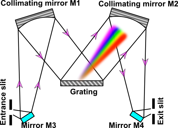
Monochromators are the most widely used dispersive instruments. They isolate a small wavelength band from a polychromatic source. Monochromators consist of a dispersive element (prism or grating) and an image transfer system (entrance slit, mirrors or lenses, and exit slit). In the Czerny-Turner monochromator, incident radiation passes the entrance slit and strikes the plane folding mirror M3 and is reflected to the concave mirror M1. Note that the entrance slit is located at the focus of M1. Thus, the beam reflected from M1 is parallel (i.e., M1 serves as a collimating element). The parallel radiation from M1 strikes the dispersion element, a grating in this case. The grating spatially disperses the spectral components of the incident radiation. Collimated rays of diffracted radiation strike the concave focusing mirror M2, are reflected to the folding plane mirror M4, and are focused on the exit slit.

Diffraction Grating

General Applications

The diffraction grating is an optical component used to spatially separate polychromatic light (white light) into its constituent optical frequencies. A simple grating consists of glass substrate with a series of parallel, equispaced lines on the front surface of the glass. Diffraction gratings are used in such diverse fields as spectroscopy, colorimetry, metrology, and laser optics.

The Diffraction Grating

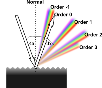
In the most general case, when a monochromatic wave is incident on a grating, with spacing d, at angle a, there will be a path difference between the ray that is reflected from one point and the ray that is reflected from a second point at distance d from the first. At the time at which the first ray hits the gating, the second ray has a path of d⋅sin(a) to the grating, and at the time that the second ray hits the gating, the first ray will have already crossed a path of d⋅sin(b), as shown schematically in Figure 2. Correspondingly, this path difference will be:

$$ \textit{path difference} = d \cdot (\sin a \pm \sin b) $$

If and only if this path difference is equal to any integer value of the wavelength does constructive interference occurs, according to the grating equation:

$$ d \cdot (\sin a \pm \sin b) = m \cdot l $$

where a is the angle of incidence, b is the angle of diffraction, d is the distance between adjacent grooves, m is the order of diffraction (integers 1, 2, 3 etc.), and ℓ is the wavelength of the incident beam.

Figure 2: Schematic of a monochromatic beam incident on a diffraction grating at angle a and diffracted at angle b. The grating spacing is the distance d.

The performance of a simple diffraction grating can best be shown with reference to Figure 2. Notice that the optical beam enters the periodic pattern (spatial fringe pattern) with a particular angle of incidence. The beam then separates into one or more "orders", according to equation (6).

Three characteristics of the simple diffraction grating stand out. First, as Figure 2 shows, the zero order is not diffracted and therefore continues undisturbed (but with some loss of power). Second, for a given wavelength, the amount of beam turning is a function of the groove period and of the angle of incidence. Finally, no real diffracted beam exists when the wavelength is greater than twice the groove period. However, when the groove period is large compared to the wavelength many orders can exist. Indeed, Indeed, Echelle gratings often operate over hundreds of orders.

Diffraction by periodic fringe pattern — Figure 3: Diffraction by the periodic fringe pattern.

Dispersion:

It is clear from the grating equation (6) that the condition for the formation of a diffracted order depends on the wavelength of the incident light. To consider the formation of a spectrum we need to know how the angle of diffraction varies with the incident wavelength. This is found by differentiating the equation with respect to b, assuming that the angle of incidence is fixed:

$$ \frac{db}{dl}=\frac{m}{d \cdot \cos(b)} $$

The quantity db/dℓ is the change of the diffraction angle corresponding to a small change of wavelength. This is known as the angular dispersion of the grating. It is greater for smaller groove spacings, d (greater number of lines per millimeter); larger orders, m; and larger diffraction angles, b.

A particularly useful grating configuration is that of the "Littrow" case, in which the diffracted beam returns along the incident beam. In this case a=b, so that the grating equation reduces to Bragg's law:

$$ 2d \cdot \sin (b) = m \cdot l $$

and the angular dispersion becomes:

$$ \frac{db}{dl} = \frac{2\tan(b)}{\lambda} $$

The linear dispersion of a grating is the product of this term and the effective focal length, f, of the system:

$$ \textit{linear dispersion} = \frac{db}{dl} \cdot f $$

Normally, we use the reciprocal linear dispersion, which gives the wavelength dispersion in nm/mm of slit width:

$$ \textit{reciprocal linear dispersion} = \textit{linear dispersion}^{-1} = \frac{dl}{db} \cdot f^{-1} $$

For example: Calculate the reciprocal linear dispersion at 500 nm wavelength of a simple grating system employing a 1200 groove/mm grating (period = d = 0.833 µm), 200 mm focal length imaging mirror, and operating in the first order with an angle of incidence of 25 degrees. Using the grating equation (6), b = 10.23 degrees. Using the angular dispersion equation (9), db/dℓ = 0.00122 rad/nm. From the linear dispersion equation (10), the linear dispersion = focal length x db/dℓ = 0.2438 mm/nm. Further, from equation (10), reciprocal linear dispersion = 4.1 nm/mm.

Bandpass and Resolution

The bandpass, s, is the width of the spectrum passed by a monochromator when illuminated by a light source with a continuous spectrum. For large bandpasses, compared with the resolution, the bandpass is given by the product of the reciprocal linear dispersion and the slit width, w:

$$ s = \textit{reciprocal linear dispersion} \cdot w = \frac{d \cdot \cos(b)}{m} \cdot \frac{w}{f} $$

The bandpass may be decreased by reducing the width of the slit until a limiting bandpass is reached. The limiting bandpass is called the resolution of the instrument. It is easy to determine this resolution by using the small-angle approximation, where b → db:

$$ s = \frac{dl}{db} \cdot \frac{w}{f} = \frac{dl}{db} \cdot \sin(db) \simeq \frac{dl}{db} \cdot db = dl \quad \Rightarrow \quad dl = \frac{d \cdot \cos(b)}{m} \cdot \frac{w}{f} \simeq \frac{d}{m} \cdot \frac{w}{f} $$

where dℓ is the resolution.

In spectral analysis, the resolution is a measure of the ability of the instrument to separate two spectral lines that are close together. Only when the resolution is smaller than the difference between the two lines can they be distinguished; if resolution is larger, the two lines will not be distinguishable.

For example: Calculate the resolution of a grating system employing a 1200 groove/mm grating (period = d = 0.833 µm), 200 mm focal length imaging mirror, and operating in the first order, with 25 µm slit. From equation (13), b = sin^-1(w/f) = 0.000125 rad; cos(b)=1.00 ; and dℓ = 0.104 nm.

Diffraction Orders

Since light of different wavelengths are diffracted at different angles, each order is drawn out into a spectrum. Each spectrum is composed of monochromatic images of the incident bundle, with the blue image nearer to the central axis. However, if monochromatic light is incident on the grating, several output beams are generated. This type of device (i.e., a beamsplitter) can be used for the generation of multiple lasers. The number of orders that can be produced by a given grating is limited by the grating constant d, because it cannot exceed 90 degrees. The highest order is given by d/ℓ. Consequently a coarse grating (with large d) produces many orders, whereas a fine grating may produce only one or two.

Free Spectral Range

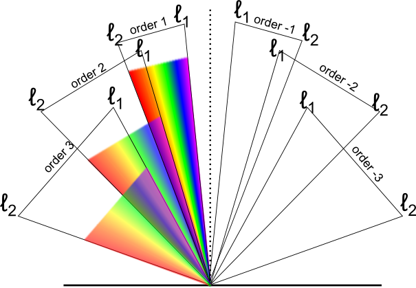
The free spectral range of a diffraction grating is defined as the largest bandwidth in a given order that does not overlap the same bandwidth in an adjacent order. If, as shown in Figure 3, ℓ₁ and ℓ₂ are the extremes of the spectrum band, then overlap will occur at the long wavelength end of the spectrum when ℓ₂ in order m is diffracted at the same angle as in order m+1. Conversely, overlap will occur at the short wavelength end when ℓ₁ in order m coincides with ℓ₂ order m-1. To avoid overlap, ℓ₂ − ℓ₁ ≤ ℓ₁/m or ℓ₂ − ℓ₁ ≤ ℓ₂/(m−1).

However, since ℓ1 < ℓ2, the free spectral range is equal to the shortest wavelength in the allowed bandwidth divided by the order number: That is, ℓ₂ − ℓ₁ ≤ ℓ₁/m.

overlapping of the spectral orders — Figure 4: Diagram depicting overlap of the spectral orders.

Efficiency

Various types of diffraction gratings have different efficiencies versus wavelength characteristics. Classical ruled gratings usually peak with very high efficiency at a certain wavelength and become rapidly less efficient upon deviation from that wavelength. Blazed holographic gratings have similar properties. On the other hand, standard holographic gratings have very little variation in efficiency over the spectral range. Classically ruled gratings, which are ruled mechanically by cutting grove after grove into a substrate with a diamond tool, are characterized by a blaze wavelength and a groove density. The blaze wavelength is the wavelength at which the grating is at its maximum efficiency. Groove density is the number of grooves per millimeter on the grating surface. The useful range of a grating can be described by the 2/3 - 3/2 rule, which simply states that the range of a grating is approximately between the lower limit of 2/3ℓ_Blase and the upper limit of 3/2ℓ_Blase. Thus for a grating with a blaze wavelength of 400 nm, the useful range is 266 to 600 nm. It is not unusual to be able to operate a grating with reasonable efficiency above the "magic" 3/2 value; however, it’s not wise to operate the grating below the "magic" 2/3 value.

The specifications of the Digikrom DK480 0.5 m monochromator with 1200 or 2400 groves/mm grating that will be used in the experiment can be found here.

Photomultiplier

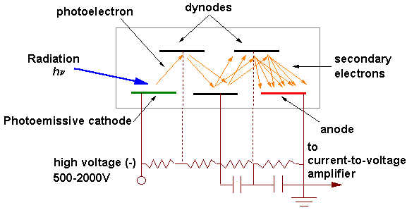
A photomultiplier (PMT) consists of a photocathode and a series of dynodes in an evacuated glass enclosure (Figure 5). Photons that strike the photoemissive cathode emit electrons due to the photoelectric effect. Instead of collecting these few electrons (there should not be a lot, since the primarily use for PMT is for very low signal) at an anode (as is done in the phototubes) the electrons are accelerated toward a series of additional electrodes called dynodes. These electrodes are each maintained at a more positive potential. Additional electrons are generated at each dynode. This cascading effect creates 10⁵ to 10⁷ electrons for each photon that hits the first cathode, depending on the number of dynodes and the accelerating voltage. This amplified signal is finally collected at the anode, where it can be measured.

The amount of current amplification is simply the ratio of the anode output current to the photoelectric current from the photocathode. Ideally, the current amplification, μ, of a photomultiplier tube having n dynode stages and an average secondary emission ratio, δ, per stage is:

$$ \mu = \delta^n $$

The secondary electron emission ratio, δ, is given by:

$$ \delta = A \cdot E^{\alpha} $$

where A is a constant, E is an interstage voltage, and α is a coefficient determined by the dynode material and geometric structure. It usually has a value of 0.7-0.8.

When a voltage V is applied between the cathode and the anode of a photomultiplier tube having n dynode stages, the current amplification, μ, becomes:

$$ \mu = \delta^n = (A \cdot E^{\alpha})^n = \bigg[A \cdot \Big( \frac{V}{n+1}\Big)^{\alpha}\bigg]^n = A^n \cdot \Big( \frac{V}{n+1} \Big)^{\alpha \cdot n} = k \cdot V^{\alpha \cdot n} $$

Typically, a PMT will have the following characteristics:

Wavelength range: 110-1100 nm (wavelength sensitivity depends on photocathode type; UV-sensitive PMTs must have UV-transmitting windows).
Quantum efficiency (Q.E.): 1-10% (Q.E. is equal to the number of electrons ejected by the photocathode divided by the number of incident photons).
Response time: 1-15 ns.

In the experiment, you will use a photomultiplier tube R928 from Hamamatsu Corporation.

Download the datasheet for the PMT here and look at the "Typical Spectral Response" diagram. Make sure you understand, in general, how spectral response relates to our experiment. and how does it relate to our experiment.

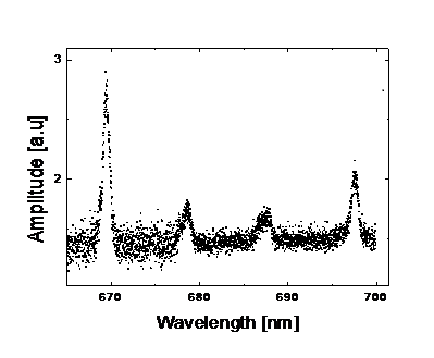
Measurements example

Here is a typical example of how measurements appear in this experiment:

Conclusions and additional important information.

The computer constantly changes the monochromator exit wavelength and records the voltage from the photomultiplier.
Bohr's formula for the Rydberg constant is in perfect agreement with experimental data (you have to demonstrate this!). However, Bohr's theory could not be extended successfully to helium or other atoms with more than one electron. You can find additional information about the hydrogen atom spectrum in any handbook on physical chemistry (see the literature section).
We recommend use of Origin or Mathematica programs to analyze the data. Mathematica is available via the Citrix server. If you are a first time user, click here for an explanation. In sections 4 and 5 you can download files containing data similair to the data obtained in the experiment.
Balmer series of hydrogen atom (unzip the file)
Dispersion of monochromator (unzip the file)
Additional information regarding monochromator and photomultiplier structure and principle of action, can be found in the references in the literature section.